機器學習基石(上)
原版的講義做得十分精美,可以很快了解
Chap01 Introduction
課堂討論:學習的定義
- 從不會到會
- 從會到更進步、熟練
課堂討論:學習的方法
- 以「樹的定義」為例
- 如何寫出「能判斷是否是樹」的程式?
- define trees and hand-program: difficult
- learn from data by observation and recognize: more easier(機器「自己」學習)
課堂討論:兩種學習方法
- 電腦: learn from data -> get knowledge by observing
- 人腦: learn from teachers -> get the essence of the knowledge(can computer do that?)
key eassence of ML
- 存在「潛藏模式」可以學習
- 若認為有「潛藏模式」,才需要學習
- 無法簡單定義
- 有可提供學習的資料
ML使用時機
- 人類無法操作
- 火星探索
- 難以定義的問題
- 視覺/聽覺辨識
- 需要快速判斷
- 股票炒短線程式
- 大量資料
- 個人化使用者體驗
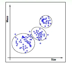
ML應用
推薦系統
將物品分解成各個porperty factors,形成vector,並與自己的喜好vector比較
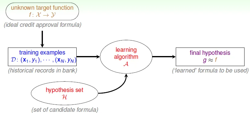
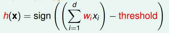
formalize the learning problem
- target funcion
f- unknown pattern to be learned
- data
D- training examples
- hypothesis set
h- candidate functions to be choosed
- hypothesis
g- best candidate function which is learned from data
- use algorithm(A) with data(D) and hypothesis set(H) to get g
![]()
Machine Learning:
use data to compute hypothesisgthat approximates targetf
Differences
Machine Learning & Data Mining
ML: the same as above
DM: use huge data to find property that is interesting
Machine Learning & Artificial Intelligence
AI -> compute something that shows intelligent behavior
ML can realize AI
traditional AI -> game tree
ML -> learning (techiniques) from board data
Machine Learning & Statistics
Statistics: use data to make inference about an unknown process
-> many useful tools for ML
課堂討論:Big Data
- As data getting bigger, the way to deal with data has to be changed.(such as distributed computation)
- not a new topic
- marketing buzz word
課堂討論:Maching Learning & Neural Network - A technique used in early AI and ML
Chap 02 Perceptron(感知器)
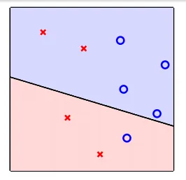
yes/no question by grading
用feature(特質)來分隔兩種不同的結果
- x: input
- w: hypothesis
- x是在d維度空間的點(d個features),w為分隔此空間的線(平面)的法向量
![]()
- 以二維空間為例:w產生的線分隔兩邊
![]()
- 也就是h(x)的正負,w所在的那一側為正
![]()
- 也就是h(x)的正負,w所在的那一側為正
select g from h
Difficult: h is infinite
Idea: 從某一條線開始,進行更改(local search)
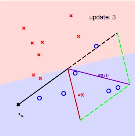
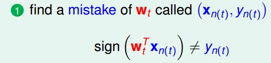
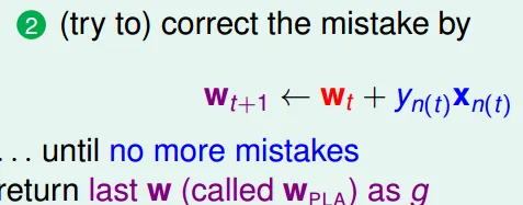
Perception Learning Algorithm(PLA)
A fault confessed is half redressed(知錯能改)
- find a mistake(which sign is wrong)
![]()
- correct the mistake
![]()
- if real ans = +, new w = w + x(使w靠近正的點)
- if real ans = -, new w = w - x(使w遠離負的點)
- keep doing until no mistake
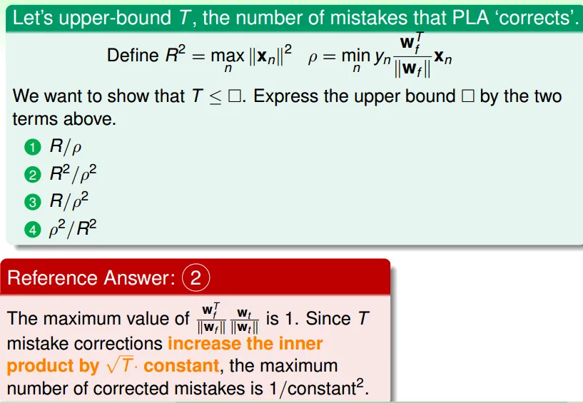
question
同乘$y_nx_n$ 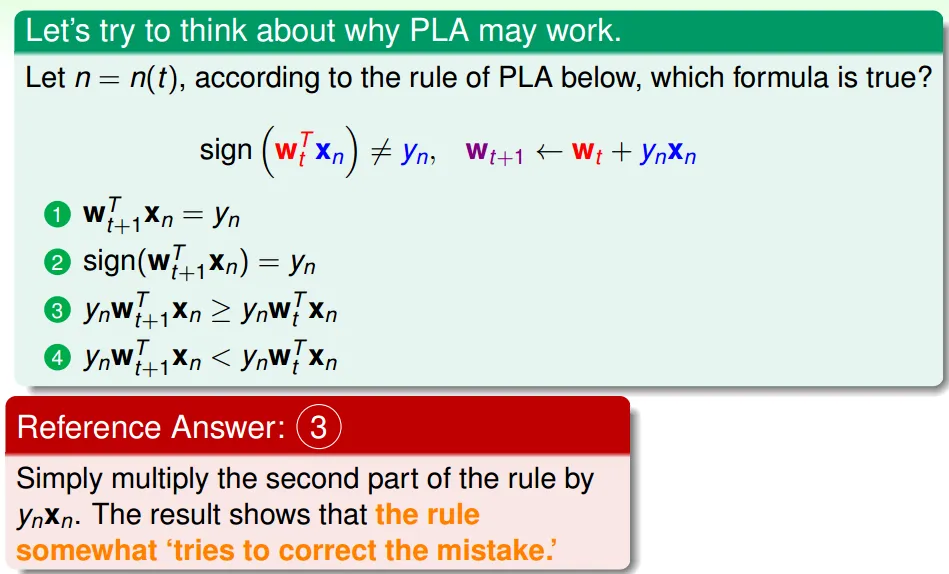
可看出錯誤變少:正確的時候,$w_nx_n$和$y_n$同號,所以$w_nx_ny_n$是正的
linear seperability

- linear seperable
- exist perfect w makes $sign(y) = sign(w_nx_n)$, n = 0~N
- 用直線(平面)必可分成無錯誤的兩塊
- if Data is linear seperable, then PLA can generate w to make no mistake
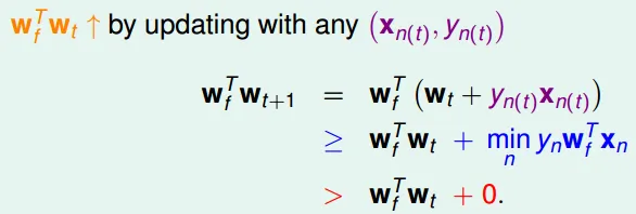
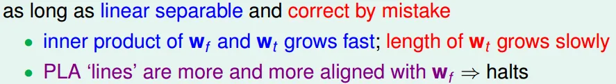
- 每次改動使$w_f$(正解)和$w_t$的內積變大,也就是愈來愈接近
![]()
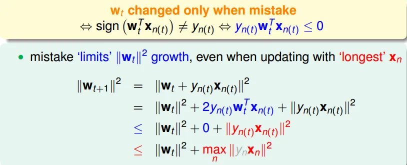
- 但成長速度有限
![]()
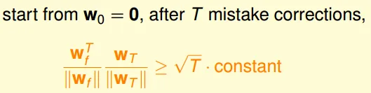
- $|W_t| <= sqrt(t) max(X_n)$
![]()
- 但成長速度有限
question
PLA Guarantee
- advantage
- simple to implement
- fast
- disadvantage
- not fully sure how long it will take
- assume linear seperable
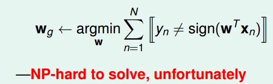
- What if no linear seperate?(in reality)
- 選出犯錯最少的
- 這是個NP-HARD問題…
![]()
Pocket Algorithm(a little modified by PLA)
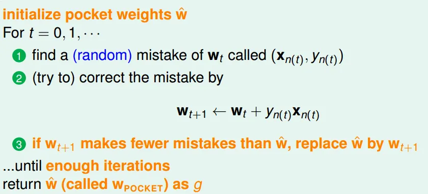
- greedy
- may not be the best answer: 可能是局部最佳解
- slower than PLA(need to compare Wt+1 and Wt)
Chap03 types of learning
Different Output Space
Binary Classification
- yes/no
- core problem to build tools
Multiclass Classification(N output class)
- Regression(迴歸分析)
- output 為一數字
- Ex. temperature, stock price
- core problem to build statistic tools
- Structured Learning
- output $y$ = structures with implicit class definition
- too many class → structure
- Ex. Speech parse tree, sequence tagging(標詞性), protein folding
Different Data Label
Supervised Learning(監督式學習)
- data with pairs of input and output
Unsupervised Learning
- doesn't have output data(沒正確答案)
- clustering(分群問題)
- density estimation(find traffic dangerous areas)
- unusual detection(find unusual data)
- usually used in data mining
![]()
Semi-Supervised
- given small amount of data with output, find output of other data
- Ex. facebook face identifier
- leverage unlabeled data to avoid 'expensive' labeling
Reinforcement Learning(增強學習)
- natural way of learning(行為學派)
- learn with 'seqentially implicit output'
- if output is good, give reinforcement
- probability of this input increases
- if output is bad, give pushnishment
- probability of this input decreases
- Ex.
- train a dog
- online ADs
- chess AI
- 和gene algorithm類似
Different Protocol
Batch Learning
- learn from known data
- duck feeding(填鴨式)
- very common protocol
Online Learning
- sequential, passive data(不斷的得到新資料)
- Every datum can improve
g - PLA, reinforcement learning is often used with online learning
- Ex. spam filter
Active Learning
- strategically-observed data
- machine can ask question(take chosen(input, output)pair to learn)
- 關於自己不會(錯誤)的問題,拿相關的資料來學習
- 比對有自信的答案(= 對答案)
Different Input Space
Feature <-> Input
Concrete Features
- each input class represents some 'sophisticated physical meaning'
- input 和 output 有相關(經過人類分類過)
Raw Features(未處理的資料)
- 'simple physical meaing' -> difficult to learn
- Ex. Digit Recognition
- concrete feature: symmtry, density
- raw feature: matrix of image bits
Abstract Features
- 'no physical learning' -> the most difficult to learn
- need 'feature conversion'
- Ex. Rating Prediction Problem
- 從歌曲評分抽出feature: 喜好, 歌的性質......
In general machine learning, those three feature types will be used
Chap 04 Feasibility of Learning
- learning will be stricted by limited data(no free lunch)
- learning from D (to infer something outside D) is doomed
Statistics
- Real environment -> unknown
- Sample data -> known
- Can sample represent the real?
- 有極小可能無法代表real status
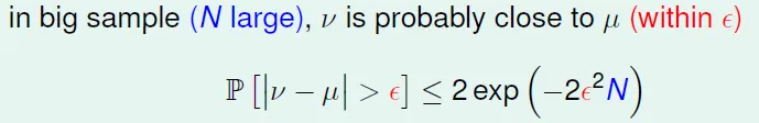
Hoeffding’s Inequality
- v and u are error rate of certain h in sample and real data
![]()
- larger sample size N or looser gap(誤差)
- higher probability to approximate real
Error between hypothesis and target function can be inferred by data 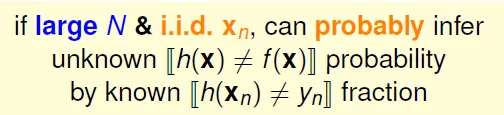
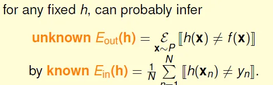
Ein and Eout
in-sample error(Ein) and out-of-sample error(Eout)
Guarantee: for large N, Ein(h) ~= Eout(h) is probably approximately correct (PAC) 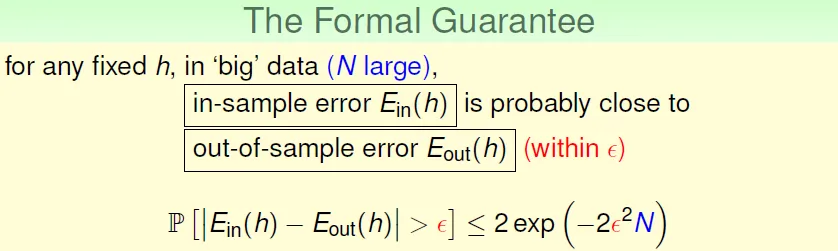
Q: if 150 people flips a coin 5 times, and one of them gets 5 heads. A: Probability is > 99% 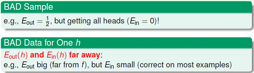
→ 做愈多次,遇到的BAD sample(Eout 和 Ein 差很多; sample和實際差距過大)的機率愈大
→ Real learning: Algorithm choose the best h which has lowest Ein(h) among H
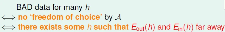
- Bad Data for a
H- 存在
h使 Ein(h) 和 Eout(h) 相差很大![]()
- 由 hoeffding 知道抽到bad data的機率很小
- 存在
- hypothesis的個數愈多,抽到BAD data的機率愈高
![]()
- 安全的data(在任何h都不是bad data)的比例 若很高,則學到的東西可能不好
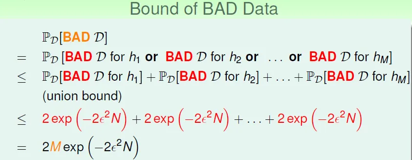
若hypothesis set的大小是有限的話,只要N夠大,Eout ~= Ein
但perceptron不是finite(有無限多種分隔可選)
Chap05 Training versus Testing
g is similar to f ↔ Eout(g) ~= Ein(g) ~= 0
But need train and test 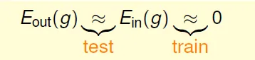
- Train: find hypothesis that can fit sample data
- Test: take good sample data that is similar to exact data
How to decide the number of hypothesis set
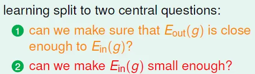
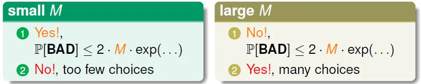
Cannot both satisfied!
Todo: Find a finite value $m_H$ can replace infinite M
Idea: M is overestimated, we use classification:
how many lines => how many kinds of line(that makes different output)
This method is called Dichotomies(二分法): Mini-hypotheses
| input | types of lines |
|---|---|
| 1 | 2 |
| 2 | 4 (00, 01, 10, 11) |
| 3 | 8 |
| 4 | 14 (2 lines that is not linearly seperable) |
| N | effective(N) <= $2^N$ |
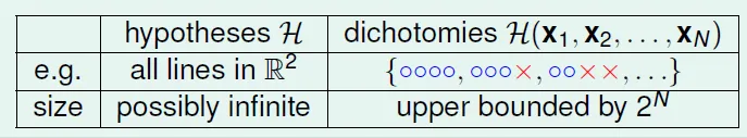
Growth Function $m_H$ = max number of dichotomies(max number of different outputs)
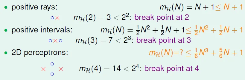
Types of Growth Function
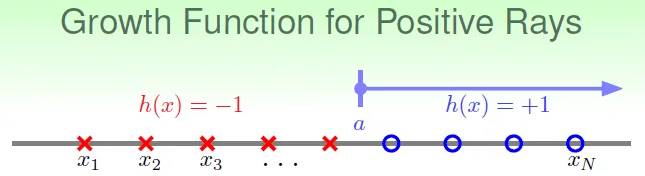
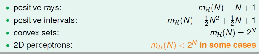
- Positive Rays
![]()
- $m_H(N)$ = N + 1
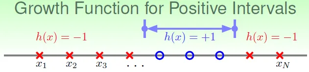
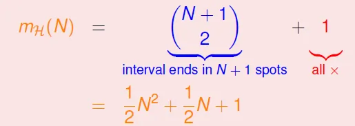
- Positive Intervals
![]()
- $C^{N+1}_2 + 1$
![]()
- $C^{N+1}_2 + 1$
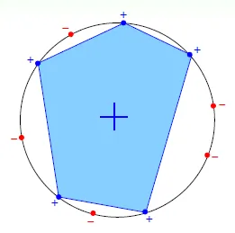
- Convex Sets
- worst case: every point make a circle
![]()
- $m_H(N) = 2^N$ -> exists N inputs that can be shattered(所有output皆可產生)
- worst case: every point make a circle
Now $m_H(N)$ is finite, but exponential
Question:Can we find polynomial instead of exponential?
Break Point of H
if all possible k inputs can't be shattered by H
k = break point for H 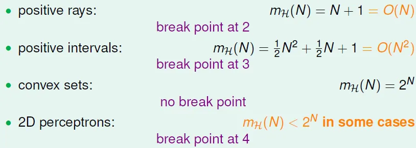
2D perceptrons: break point at 4
3 inputs: exist at least one input that can shatter 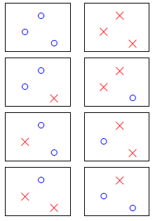
4 inputs: for all inputs, no shatter
If there is no breakpoint, we can only find exponential($2^N$) increase
If there is a breakpoint, we can find polynomial($O(N^k)$)increase
breakpoint愈小,hypothesis set 成長的速度受到愈多限制(因為無法shatter,所以hypothesis數比exponential小)
Chap06 Theory of Generalization
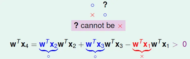
Q: maximum possible $m_H(N)$ if input number(N) = 3 when breakpoint(k) = 2?
A: x1, x2 cannot shatter, and so does x2, x3 and x1, x3 
→ When N > breakpoint, break point restricts $m_H(N)$ a lot!
idea: prove $m_H(N) \leq$ poly(N) if N > k
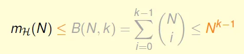
Bounding function
bounding function B(N, k): maximum possible $m_H(N)$ when break point = k
Table of bounding function(incomplete) 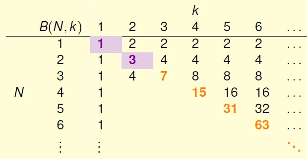
B(N, k) = $m_H(N) = 2^N$ when N < k(shatter)
B(N, k) < $m_H(N) = 2^N - 1$ when N = k(至少比shatter少一種)
When N > k :Using reduce, Ex. B(4,3) 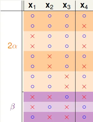
α: dichotomies on (x1, x2, x3) with x4 paired
β: dichotomies on (x1, x2, x3) with x4 no paired
Because B(4,3) can't shatter any 3 inputs
→ α + β can't shatter at (x1, x2, x3)
→ α + β $\leq$ B(3,3)
Because B(4,3) can't shatter any 3 inputs and x4 is already paired
→ α can't shatter any 2 inputs at (x1, x2, x3)
→ α $\leq$ B(3,2)
B(4,3) = 2α + β $\leq$ B(3,3) + B(3,2)
Generalized: B(N,k) $\leq$ B(N-1,k) + B(N-1,k-1) 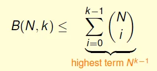
By calculation: $m_H(N) \leq B(N,k) \leq N^{k-1}$
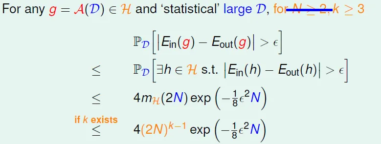
Conclusion: $m_H(N)$ is polynomial if break point exists for N >= 2 & k >= 3!!
'<=’ can be ‘=’ actually -> not easy proof(skipped)
Vapnik-Chervonenkis (VC) bound
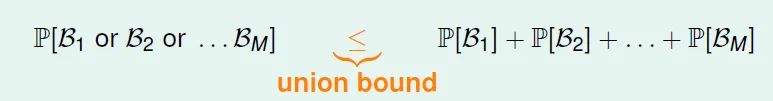
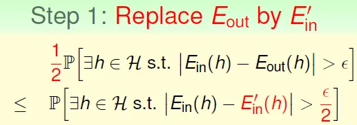
Proof: BAD Bound for General H
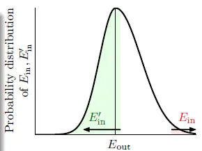
- Now Ein(h) finite, but Eout(h) still infinite(Eout的點有無限個)
- use ghost sample data Ein' to replace(想像再sample一次會產生的Ein',將這段資料作為eout)
- 圖中Ein離Eout很遠,是bad data,只要Ein'在Eout附近,Ein'也會離Eout很遠
![]()
- Eout 乘1/2,使其成為不等式
![]()
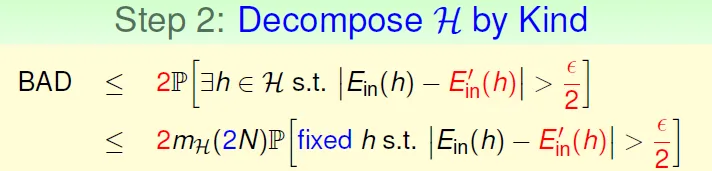
- 將bad data相似的hypothesis分在一起
- 總共有2N個data(Ein + Ein') → $m_H(2N)$
![]()
- 因為有了$m_H()$函數,變成只考慮固定的hypothesis
- 總共有2N個data(Ein + Ein') → $m_H(2N)$
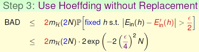
- Use Hoeffding without Replacement
- 可視為2N個點取N個點,sample為Ein,剩下為Ein'(不放回去)
- 使用 'Hoeffding without Replacement': 公式和hoeffding 一樣
![]()
- Hoeffding只用於單一hypothesis,所以需要步驟2
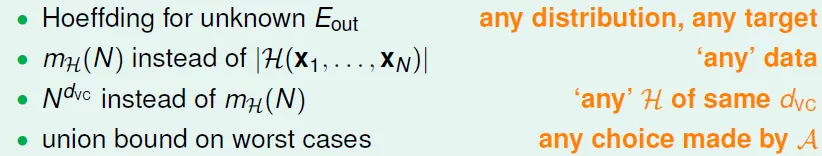
Vapnik-Chervonenkis (VC) bound 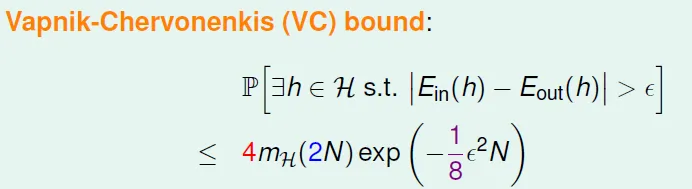
→ proved that learning with 2D perceptrons feasible!
You need to let everything good to learned well 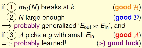
Chap 07 VC Dimension
VC Dimension
= maximum non-break point = (minimum k) - 1
= largest N that can shatter
2D perceptron review 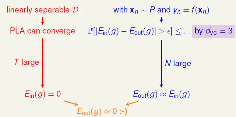
How does PLA in more than 2 dimension?
- 2D → 3
- d-dimension perceptron
- d_VC = d+1
Proof
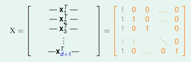
- d_VC > d+1 → d+1 can shatter
input matrix which is invertible![]()
for any y, we can find w such that sign(Xw) = y → $w = yX^{-1}$ → it can shatter - d_VC < d+1 → d+2 can't shatter
linear dependence restricts dichotomy![]()
if row > column, it would cause linear dependence![]()
for any input, we can find some $a_n$ that makes an output can't happen → no shatter![]()

freedom
dimension, number of parameters, hypothesis quantity(M) → degrees of freedom
d_VC(H) = effitive binary degrees of freedom = powerfulness of H
The more powerful it is (d_vc bigger), the more probability to get bad data 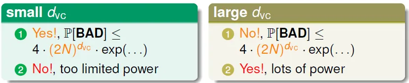
question: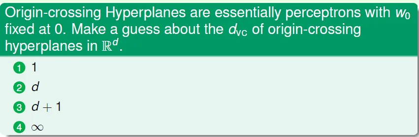
比perceptron少一個parameter → d
penalty for model complexity 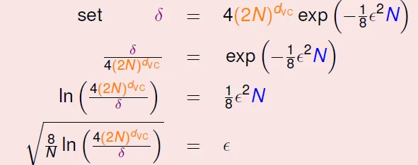
model愈強,Ein愈小,和Eout誤差愈大 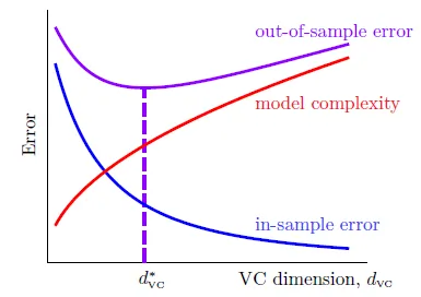
number of data(N) should be 10000 d_vc in theory; 10 d_vc is enough in practice, because VC bound is loose 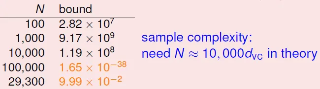
question: 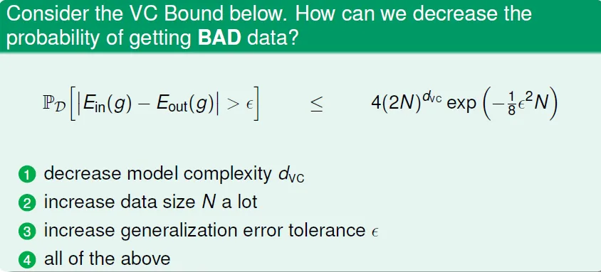
all of above(increase power of model)
Chap08 Noise and Error
- Noise in y
- Example: good customer mislabeled as bad
- Noise in x
- Example: incorrect feature calculation
- Would get probabilisic output y ≠ h(x) by given P(y|x)
Does VC bound works in noise? Yes, if i.i.d.(Independent and identically distributed) 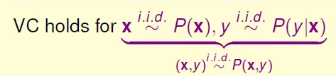
→ we can view as 'ideal mini-target' + noise
→ learning goal is to predict ideal mini-target(which is Y that has high P(Y|X) given X) on often seen inputs(X with high P(X))
Eout use expectation instead of Σ , $err$ means pointwise error(only consider a point x) 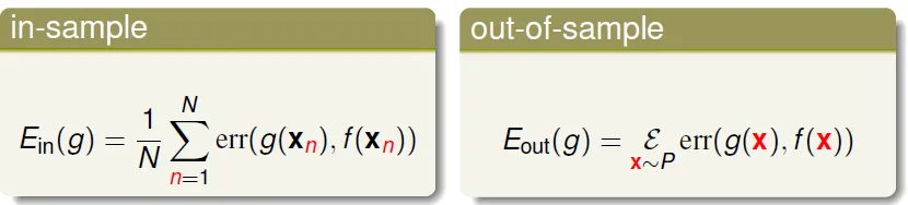
Error Measure
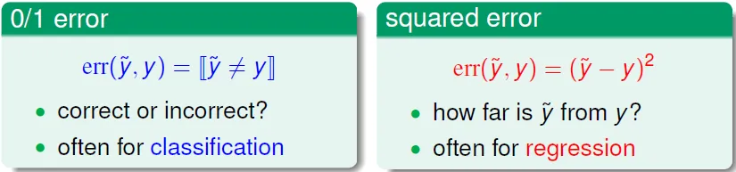
- classification(0/1 error)
- minimum flipping noise(最少錯誤的output)
- NP-hard to optimize
- regression use squared error
- minimum gaussian noise(output和正確答案的平方差最小)
Error is **application/user dependent **
- CIA fingerprint login error
- not allow predict 0 to 1
![]()
- not allow predict 0 to 1
- Supermarket member login error
- not want to predict 1 to 0
- error weight is not the same!
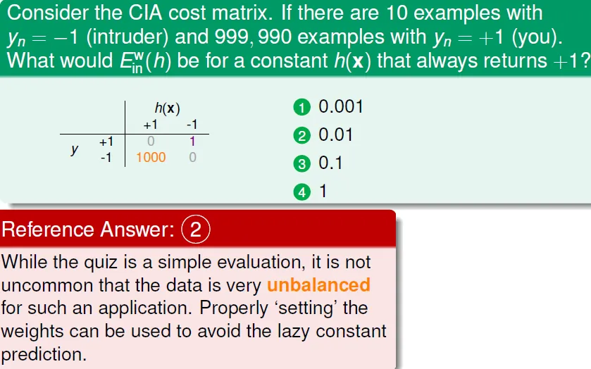
Example: pocket
- modify Ein to $E^w_{in}$(with weight)
- weight愈高的錯誤愈容易被選來修正
權重可以套用在許多機器學習的演算法
algorithm choosing
Algorithmic Error Measures $\hat{err}$
- True
- error cannot be ignored or created
- plausible(可用性)
- 0/1 error
- squared error
- friendly(較容易的演算法)
- close form solution(有公式解,如Chap09的linear regression)
- convex objective function(可以持續更新的,如PLA)
- $\hat{err}$ is key part of many algorithms
參考資料
Coursera機器學習基石
C老師上課講解