電腦對局理論

註：此為2014年版，且只寫到第八章(因為教授只考到這)

Introduction

學習電腦對局的用處

1. 電腦愈聰明，對人類愈有用
2. 電腦學得的技巧讓人學習

為何學棋局

1. 容易辨別輸贏
2. 規則簡單(先備知識少)

圖靈測試(Turing test)

If a machine is intelligent, then it cannot be distinguished from a human

• 反過來利用的例子 - CAPTCHA(驗證碼): Completely Automated Public Turing test to tell Computers and Humans Apart
• Wolfram Alpha
  • knowledge base of Siri

Problems

• Are all human behaviors intelligent?
• Can human perform every possible intelligent behavior?
  → Human Intelligence 和 Intelligence 並不完全相同

改變目標

• From Artificial Intelligence to Machine Intelligence
  • machine intelligence: the thing machine can do better than human do
• From imitation of human behaviors to doing intelligent behaviors
• From general-purpose intelligence to domain-dependent Expert Systems

重大突破

• 1912 - End-Game chess playing machine
• ~1970 - Brute Force
• 1975 - Alpha-Beta pruning(Knuth and Moore)
• 1993 - Monte Carlo

無關：核心知識

用少部分的核心知識(要記得的事物)推得大多數的知識
Ex. 背九九乘法表推得所有多位數乘法
建構式數學(X)

對局分類

研究遊戲之前的必要分析：分類

By number of players

• Single-player games
  • puzzles
  • Most of them are NP-complete
    • or the game will be not fun to play
• Two-player games
  • Most of them are either P-SPACE-complete(polynomial space usage) or exponential-time-complete
    • PSPACE-complete can be thought of as the hardest problems in PSPACE, solution of PSPACE-complete could easily be used to solve any other problem in PSPACE
• Multi-player games

By state information obtained by each player(盤面資訊是否完全)

• Perfect-information games
  • all players have all the information to make a correct decision
• Imperfect-information games
  • some information is only available to selected players, for example you cannot see the opponent's cards in Poker(不知對手的牌或棋子, Ex. 橋牌)

By rules of games known in advance(是否有特殊規則、是否知道對手的行動)

• Complete-information games
  • rules of the game are fully known by all players in advance
• Incomplete-information games
  • partial rules are not given in advance for some players(Ex. 囚犯困境賽局)

definition of perfect and complete information in game theory

By whether players can fully control the playing of the game(是否受隨機性影響)

• Stochastic games
  • there is an element of chance such as dice rolls
• Deterministic games
  • players have a full control over the games

Example(not fully sure):

• perfect-information complete-information deterministic game: chinese chess, go
• perfect-information complete-information stochastic game: dark chinese chess, 輪盤(Roulette)
• perfect-information incomplete-information deterministic game: Prisoner’s Dilemma
• perfect-information incomplete-information stochastic game: ?
• inperfect-information complete-information deterministic game: ?
• inperfect-information complete-information stochastic game: monopoly, bridge
• inperfect-information incomplete-information deterministic game: battleship, bingo
• inperfect-information incomplete-information stochastic game: most of the table/computer games

Chap02 Basic Search Algorithms

• Brute force
• Systematic brute-force search
  • Breadth-first search (BFS)
  • Depth-first search (DFS)
    • Depth-first Iterative-deepening (DFID)
  • Bi-directional search
• Heuristic search: best-first search
  • A*
    • IDA*

Symbol Definition

• Node branching factor b
  • degree
  • number of neighbor vertexs of a node
• Edge branching factor e
  • number of connected edges of a node
• Depth of a solution d
  • 最短深度, D 為最長深度
  • Root深度為0
• If b and e are average constant number, e >= b(兩個點之間可能有多條線)

Brute-force search

Used information

• initial state
• method to find adjacent states
• goal-checking method(whether current state is goal)

Pure brute-force search program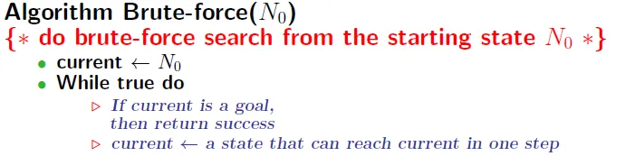

• 隨機走旁邊的一個點
• 不記憶走過的路
  • May take infinite time
• Pure Random Algorithm 應用
  • 驗證碼(e.g. 虛寶)
  • 純隨機數

BFS(Breadth-First Search)

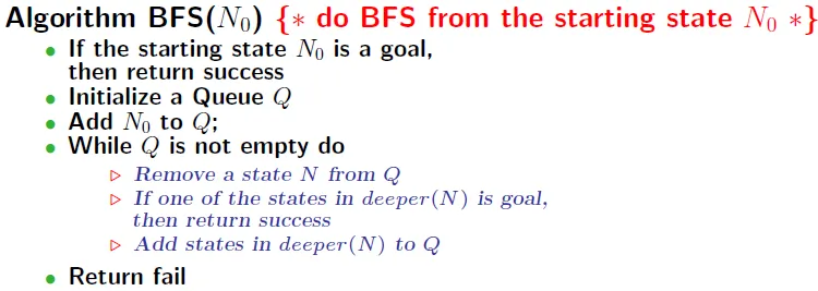
deeper(N): 回傳與N相鄰的點
record parent state and backtrace to Find the path

• Space complexity: $O(b^d)$ → Too big!

• Time complexity: $O(b^{d-1} * e)$

  • → costs O(e) to find deeper(N), at most check b^(d-1) times(deeper(leaf) do not return new node)

• Open list: nodes that are in the queue(candidate nodes)

• Closed list: nodes that have been explored(assure not answer, can skip)

  • Need a good algorithm to check for states in deeper(N) are visited or not
    • Hash
    • Binary search
  • not need to have because it won't guarantee to improve the performance
  • if it is possible to have no solution, Need to store nodes that are already visited

• node： open list → check is goal or not, explore(deeper) → closed list

Property

• Always finds optimal solution
• Do not fall into loops if goal exists(always "deeper")

Disk based algorithm

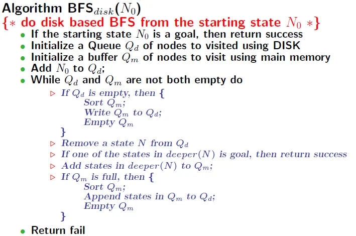
Solution for huge space complexity

• disk: store main data
• memory: store buffers

• Store open list(QUEUE) in disk
  • Append buffered open list to disk when memory is full or QUEUE is empty
• Store closed list in disk and maintain them as sorted
  • Merge buffered closed list with disk closed list when memory is full
  • delay cheking: check node in the closed list or not before being taken from open list

Disk based algorithms

• not too slow
  • read large file in sequence
    • queue(always retrieve at head and write at end)
  • sorting of data in disk
    • merge sort between disk list and buffer list
• very slow
  • read file in random order(disk spinning)
• 系統為資源和效率(時間、空間、錢)的trade-off

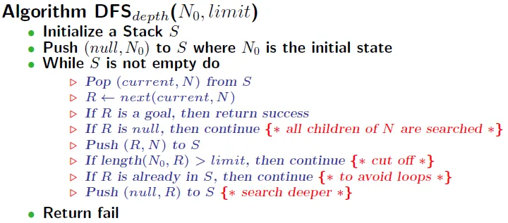
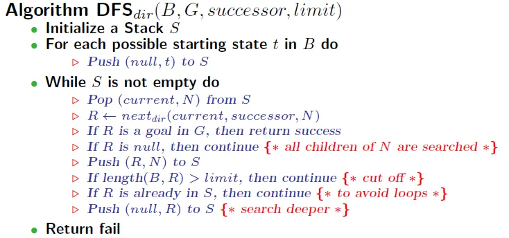
DFS

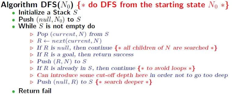
• performance mostly depends on move ordering
  • If first choose the branch include the goal, find answer quick
  • get out of long and wrong branches ASAP!
  • implement next(current, N)
    • 作用：列舉出N的所有鄰居
    • 回傳下一個N的鄰居，目前列舉到current
    • next(null, N) -> return first neighbor of N
• time complexity: $O(e^D)$
  • number of possible branches at depth D
• space complexity: $O(D)$
  • Only need to store current path in the Stack

Property

• need to store close list (BFS: do not need to)
• May not find an optimal solution
• Can't properly implement on disk
  • very huge closed list
    • Use data compression or bit-operation techniques to store visited nodes
    • Need a good heuristic to store the most frequently visited nodes to avoid swapping too often
  • need to check closed list instantly(BFS: can be delayed)
• Can DFS be paralleled? Computer scientists fails to do so even after 30 years
• Most critical drawback: huge and unpredictable time complexity

General skills to improve searching algorithm

Iterative-Deepening(ID) 逐層加深

• inspired from BFS(BFS = BFID)
• 限制搜尋時的複雜度，若找不到再放寬限制
• prevent worse cases

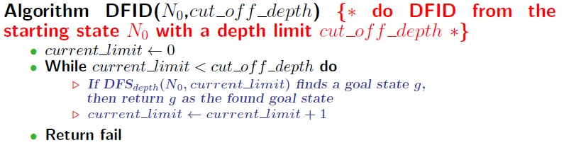
Deep First ID(DFID)

• 限制深度
  • 找到解立即return
  • 
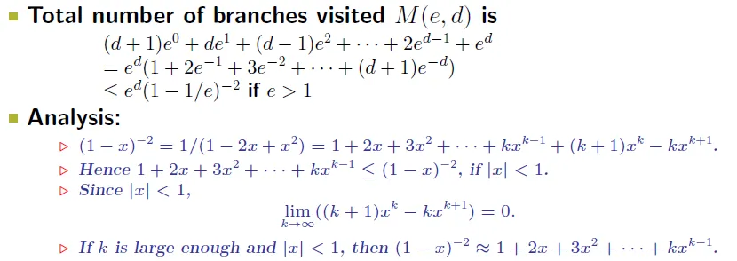
  • time complexity using 二項式定理
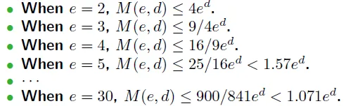
    • M(e, d) ~ $O(e^d)$ when e is sufficiently large
    • → no so much time penalty to use ID when e is big enough
  • 關鍵：設定初始限制和限制放寬的大小
  • always find optimal solution

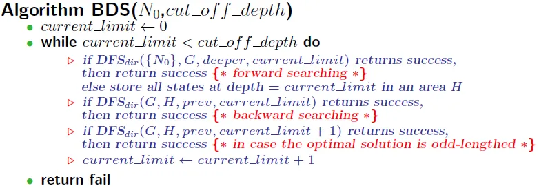
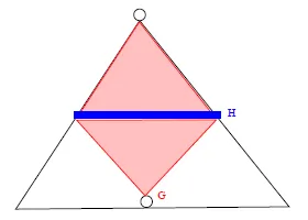
Bi-directional search

• DFSdir(B, G, successor, i): DFS with starting states B, goal states G, successor function and depth limit i

• nextdir(current, successor, N): returns the state next to the state "current" in successor(N)

  • deeper(current, N) for forward searching
    • deeper(N) contains all next states of N
  • prev(current, N) for backward searching
    • prev(N) contains all previous states of N
      

• Forward Search: store all states H

• Backward Search: find the path from G(goal) to H at depth = limit or limit+1(for odd-lengthed solutions)

• also use the concept of iterative-deepening
  

• Time complexity: $O(e^{d/2})$

  • the number of nodes visited is greatly reduced(compared with original $O(e^d)$)

• Space complexity: $O(e^{d/2})$

  • Pay the price of storing state depth(H)

• restrict

  • can't assure to find optimal solution
  • need to know what the goals are
    • bi-directional search is used when goal is known, only want to find path, like solving 15-puzzle

Heuristic(啟發式) search

Definition: criteria, methods, or principles for deciding which is the most effective to achieve some goal
→ By 經驗法則(so not always have optimal solution)

• 先走最有可能通往答案的state(good move ordering)
  • best-first algorithm : like greedy
• The unlikely path will be explored further(pruning)
• Key: how to pick the next state to explore
  • need simple and effective estimate function to discriminate

Heuristic search -- A*

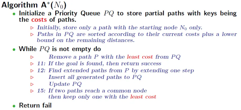
line 12: add all possible path that depth = depth + 1

• Open list: a priorty queue(PQ) to store paths with costs
• Closed list: store all visited nodes with the smallest cost
  • Check for duplicated visits in the closed list only
  • A node is inserted if
    • it has never been visited before
    • being visited, but has smaller cost

• Given a path P
  • g(P) = current cost of P
  • h(P) = estimation of remaining path to goal(heuristic cost of P)
  • f(P) = g(P) + h(P) is the cost function
• Assume all costs are positive, so there is no need to check for falling into a loop
• cost function所推測的cost不可超過實際的cost，否則不保證找到最佳解
  • if h() never overestimates the actual cost to the goal (called admissible可容許), then A* always finds an optimal solution
  • 證明？

1. h(n)=0 : A* 等同 BFS
2. h(n)<目前節點到結束點的距離 : A* 演算法保證找到最短路徑, h(n)越小, 搜尋深度越深(代表花愈多時間)
3. h(n)=目前節點到結束點的距離 : A* 演算法僅會尋找最佳路徑, 並且能快速找到結果(最理想情況)
4. h(n)>目前節點到結束點的距離 : 不保證能找到最短路徑, 但計算比較快
5. h(n)與g(n)高度相關 : A* 演算法此時成為Best-First Search
   http://blog.minstrel.idv.tw/2004/12/star-algorithm.html

Question:

• What disk based techniques can be used?
• Why do we need a non-trivial h(P) that is admissible?
• How to design an admissible cost function?

DFS with threshold

• DFScost(N, f, threshold)
  • starting state N
  • cost function f
  • cuts off a path if cost bigger than threshold

DFS1: Use next1(current,N) find neighbors of N (in the order of low cost to high cost)

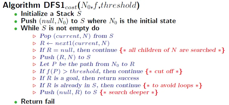
DFS2: Use a priority queue instead of using a stack in DFScost

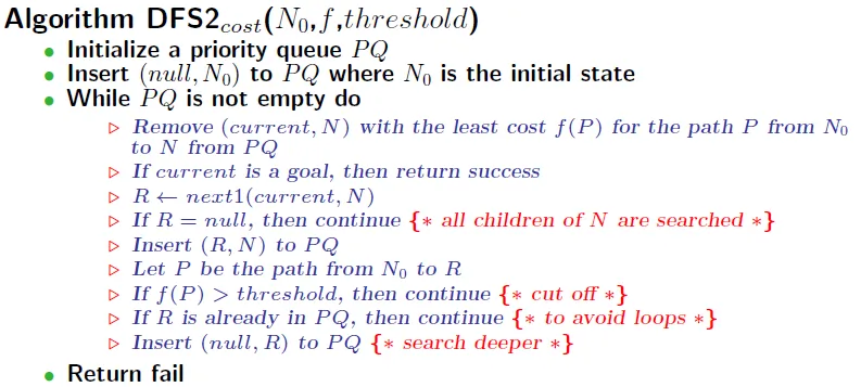
It may be costly to maintain a priority queue

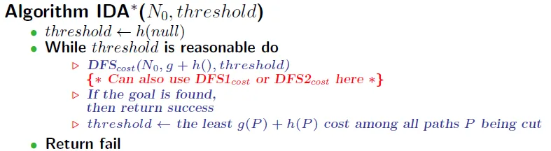
IDA* = DFID + A*

用A*的cost作為DFS的threshold

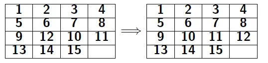
Ex. 15 puzzle
all posibilities: $16! \leq 2.1 \times 10^{13}$
g(P): the number of moves made so far
h(P): Manhattan distance between the current board and the goal
Manhattan distance from (i, j) to (i', j') is |i' - i| + |j' - j| (admissible)

basic thought for a problem

What you should think about before playing a game：

• Needed to
  • Find an optimal solution?
  • batch operations?
  • disk based algorithms?
  • Search in parallel?
• Balancing in resource usage:
  • memorize past results vs efforts to search again(time and space)
  • The efforts to compute a better heuristic(time to think a heuristic?)
  • The amount of resources spent in implementing a better heuristic and the amount of resources spent in searching(complexity of heuristic function)
• For specific algorithm
  • heuristic : How to design a good and non-trivial heuristic function?
  • DFS : How to get a better move ordering?

Can these techniques be applied to two-person game?

algorithm整理

| Name | Time Complexity | Space Complexity | OptimalSolution | UseDisk | Description |
| --------- | --------------- | ---------------- | ------------------ | ------- |
| brute | $∞$ | $O(1)$ | No | No |
| BFS | $O(b^d)$ | $O(b^{d-1} * e)$ | Yes | Needed |
| DFS | $O(e^d)$ | $O(d)$ | No | NoNeed |
| Heuristic | N\A | N\A | Yes, if admissible | -- | Ex. A* |
| BDS | $O(e^{d/2})$ | $O(e^{d/2})$ | No | Needed | DFS + bidiretional search |
| DFID | $O(e^d)$ | $O(d)$ | Yes | NoNeed | DFS + ID |
| IDA* | N\A | N\A | Yes | N\A | DFID + A* |

Chap03 Heuristic Search with Pre-Computed Databases

new form of heuristic called pattern databases

• If the subgoals can be divided
  • Can sget better admissible cost function by sum of costs of the subgoals
• Make use of the fact that computers can memorize lots of patterns
  • 使用已經計算過的 pattern 來做出更好、更接近real cost的heuristic function

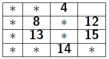
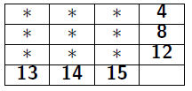
Using 15 puzzle as example

• State space can be divided into two subsets: even and odd permutations
• $f_1$ is number of inversions in a permutation X1X2...XN
  • inversion is a distinct pair Xi > Xj such that i < j(後面有幾個數比自己小)
  • Example: 10,8,12,3,7,6,2,1,14,4,11,15,13,9,5 has 9+7+9+2+5+4+1+0+5+0+2+3+2+1 inversions
• $f_2$ is the row number that empty cell is(空的那一格在哪一行)
• f = $f_1$ + $f_2$
• Slide a tile never change the parity
  • Proof: skip(a lot of)

Solving Result

• 1-MIPS machine
• 30 CPU minutes in 1985
• using IDA* with Manhattan distance heuristic

Non-additive pattern databases

• 原本cost funtion為15片個別的distance之和，若能一次計算多片的distance？
• linear conflict: 靠很近不代表步數少(如[2, 1, 3, 4]交換至[1, 2, 3, 4]並不只兩步)
  • 有可能移成pattern時，反而使其他片遠離
  • 
• Fringe(初級知識)
  • subset of selected tiles called pattern
    • tiles not selected is "don't-care tile", all looked as the same
  • If there are 7 selected tiles, including empty cell
    • 16!/9! = 57657600 possible pattern size

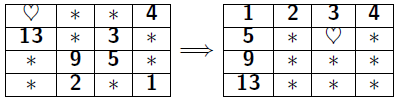
goal fringe: 選擇的方塊都和goal的位置一樣

• precompute the minimum number of moves(fringe number) to make goal fringe
  • goal fringe: 找給定的選擇方塊，在任何pattern中，最小需要移動成最終目標的步數
  • We can solve it because the pattern size is relatively small
• Pro's
  • pattern size↑, fringe number↑, which means better estimation
    • because estimate number it is closer to the real answer
• Con's
  • Pattern with a larger size
    • consuming lots of memory and time
    • limited by source
  • not optimal

Property

1. Divide and Conquer

• Reduce a 15-puzzle problem into a 8-puzzle
• 魔術方塊 -- 分成六面
• Cannot easily combine
  • affect tiles that have reached the goal in the subproblem when solving the remains

2. Used as heuristic function(admissible)

More than one patterns

• How to Find better patterns for fringes?
  • → Can we combine smaller patterns to form bigger patterns?

For different pattern databases P1, P2, P3 ...

• patterns may not be disjoint, may be overlapping
• The heuristic function we can use is
  • $h(P_1, P_2, P_3 ... ) = max{h(P_1),h(P_2),h(P_3) ...}$

How to make heuristics and the patterns disjoint?

• patterns should be disjoint to add them together(see below)
  • Though patterns are disjoint, their costs are not disjoint
    • Some moves are counted more than once

f(P1) + f(P2) is admissible if

1. f() is disjoint with respect to P1 and P2
2. both f(P1) and f(P2) are admissible

For Manhattan distance heuristic

1. Each region is a tile
   • Divide the board into several disjoint regions
2. They are disjoint
   • only count the number of moves made by each region
     • doesn't count cross-region moves

Refinement
Partition the board into disjoint regions using the tiles in a region of the goal arrangement as a pattern

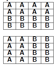
只算每個region內的片所移動的步數和，作為新定義的fringe number
如此一來，就可以將每個region的cost相加而保持admissible

Disjoint pattern

A heuristic function f() is disjoint with respect to two patterns P1 and P2 if

1. P1 and P2 have no common cells
2. The solutions corresponding to f(P1) and f(P2) do not interfere each other

Revised fringe number f'(p): for each fringe arrangement F, the minimum number of fringe-only moves to make goal fringe

Result

Solves the 15 puzzle problem using fringe that is more than 2000 times faster than the previous result by using the Manhattan distance

• The average Manhattan distance is 76.078 moves in 24-puzzle
• The average value for the disjoint database heuristic is 81.607 moves in 24-puzzle
• only small refinement on heuristic function would make performance far better

Other heuristics

• pairwise distance
  • partition the board into many 2-tiles so that the sum of cost is maximized
    For an $n^2 - 1$ puzzle, we have $O(n^4)$ different combinations
    using

What else can be done?

2. Better way of partitioning
3. Is it possible to generalize this result to other problem domains?
4. Decide ratio of the time used in searching and the time used in retrieving pre-computed knowledge
   • memorize vs compute

Chap 04 Two-Player Perfect Information Games Introductions

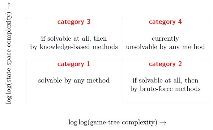
Conclusion: decision complexity is more important than state-space complexity

trade-off between knowledge-based methods and brute-force methods

Domain: 2-person zero-sum games with perfect information
Zero-sum means one player's loss is exactly the other player's gain, and vice versa.

Definition

Game-theoretic value: the outcome of a game when all participants play optimally
Game-theoretic value for most games are unknown or are only known for some legal positions.

Type	Description
Ultra-weakly solved	在初始盤面可知，遊戲中先行者或後行者誰有必勝、或必不敗之策略
Weakly solved	for the initial position a strategy has been determined to achieve the game-theoretic value(知道必不敗之策略為何)
Strongly solved	a strategy has been determined for all legal positions(任何合法情況都能知道最佳策略)

State-space complexity of a game: the number of the legal positions in a game(可能的盤面)
Game-tree complexity(decision complexity) of a game: the number of the leaf nodes in a solution search tree(可能的走法)

A fair game: the game-theoretic value is draw and both players have roughly equal probability on making a mistake.

• Paper-scissor-stone
• Roll a dice and compare who gets a larger number

Initiative(主動): the right to move first

• A convergent game: the size of the state space decreases as the game progresses
  • Example: Checkers
• A divergent game: the size of the state space increases as the game progresses
  • Example: Connect-5
• A game may be convergent at one stage and then divergent at other stage.
  • Ex. Go, Tic-Tac-Toe

Threats are something like forced moved or moves you have little choices.
Threats are moves with predictable counter-moves

Classification

Questions to be researched
Can perfect knowledge obtained from solved games be translated into rules and strategies which human beings can assimilate?
Are such rules generic, or do they constitute a multitude of ad hoc recipes?
Can methods be transferred between games?

Connection games
Connect-four (6 * 7)
Qubic (4 * 4 * 4)
Renju - Does not allow the First player to play certain moves, An asymmetric game.
mnk-Game: a game playing on a board of m rows and n columns with the goal of obtaining a straight line of length k.
Variations: First ply picks only one stone, the rest picks two stones in a ply. -> Connect 6.

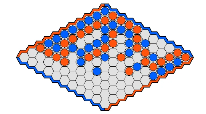
Hex (10 * 10 or 11 * 11)
Exactly one of the players can win.
solved on a 6 * 6 board in 1994.

Proof on exactly one player win
Assume there is no winner

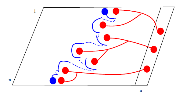
blue should totally block red at some place -> blue will connect!

let R be the set of red cells that can be reached by chains from rightmost column
R does not contain a cell of the leftmost column; otherwise we have a contradiction
let N(R) be the blue cells that can be reached by chains originated from the rightmost column.
N(R) must contain a cell in the top and bottom row , Otherwise, R contains all cells in the First/bottom row, which is a contradiction.
N(R) must be connected. Otherwise, R can advance further. Hence N(R) is a blue winning chain.

Strategy-stealing argument

made by John Nash in 1949
後手無一般化的必勝法
若後手有必勝法，則先手可以先隨機下一子(並無視之)，再照著後手的下法
後手必勝的下法包含了第一手，則再隨機下一子，將其視為第一子
限制：不能有和，下子不會有害，symmetric，history independent，

Assume the initial board position is B0
f(B) has a value only when it is a legal position for the second player.
rev(x): interchange colors of pieces in a board or ply x.
always has exactly one winner

Not Solved
Chess DEEP BLUE beat the human World Champion in 1997
Chinese chess Professional 7-dan in 2007
Shogi
Claimed to be professional 2-dan in 2007
Defeat a 68-year old 1993 Meijin during 2011 and 2012

Go
Recent success and breakthrough using Monte Carlo UCT based methods.
Amateur 1 dan in 2010.
Amateur 3 dan in 2011.
The program Zen beat a 9-dan professional master at March 17, 2012
First game: Five stone handicap and won by 11 points
Second game: four stones handicap and won by 20 points

possible to use heuristics to prune tremendously when the structure of the game is well studied

Methods to solve games
Brute-force methods

• Retrograde analysis(倒推)
• Enhanced transposition-table methods(?)
  Knowledge-based methods
• Threat-space search and lambda-search
• Proof-number search
• Depth-First proof-number search
• Pattern search
  • search threat patterns, which are collections of cells in a position
  • A threat pattern can be thought of as representing the relevant area on the board
    Recent advancements
• Monte Carlo UCT based game tree simulation
  • Monte Carlo method has a root from statistic
  • Biased sampling
  • Using methods from machine learning
  • Combining domain knowledge with statistics
• A majority vote algorithm

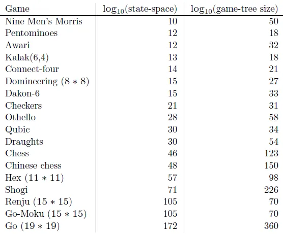
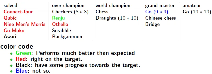
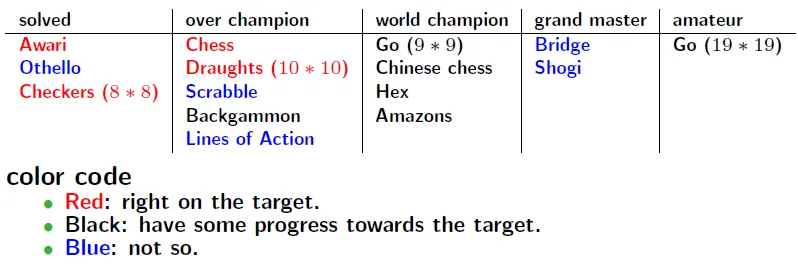
low state-space complexity have mainly been solved with brute-force methods.
Nine Men's Morris

low game-tree-complexities have mainly been solved with knowledge-based methods.
by intelligent (heuristic) searching with help of databases
Go-Moku, Renju, and k-in-a-row games

The First player has advantages.
Two kinds of positions
P-positions: the previous player can force a win.
N-positions: the next player can force a win.

First player to have a forced win, just one of the moves that make P-position.
second player to have a forced win, all of the moves must lead to(造成) N-positions

At small boards, the second player is able to draw or even to win for certain games.

Try to obtain a small advantage by using the initiative.
The opponent must react adequately on the moves played by the other player.
Force the opponent to always play the moves you expected.

Offsetting the initiative

一子棋 by 張系國 棋王 -> 先手優勢極大，隨著棋子增加，所需贏的步數就愈少。

讓子
Ex. Go k = 7.5 in 2011

Enforce rules so that the first player cannot win by selective patterns.
Ex. Renju

The one-move-equalization rule: one player plays an opening move and the other player then has to decide which color to
play for the reminder of the game.
. Hex.
. Second-player will win.

The First move plays one stone, the rest plays two stones each.
Can't prove it is fair

The first player uses less resource.
For example: using less time.
Ex. Chinese chess.

1990's prediction at 2000

2000's prediction at 2010

Chap 05 Computer chess programming by Shannon

C.E. Shannon

• 1916 ~ 2001.
• The founding father of Information theory.
• The founding father of digital circuit design.

Ground breaking paper for computer game playing: "Programming a Computer for Playing Chess", 1950.
Presented many novel ideas that are still being used today.(太神啦！)

Analysis

• typical 30 legal moves in one ply(下子)
• typical game last about 40 moves
  • will be 10^120 variations
• possible legal position(state space complexity) is roughly 10^43
• CPU speed in 1950 is 10^6 per second current CPU speed is 10^9 per second, still not fast enough to brute force it

But it is possible to enumerate small endgames
3~6 piece endgame roughly 7.75*10^9 positions

Three phases of chess

• Opening
  • Development of pieces to good position
• Middle
  • after opening until few pieces
  • pawn structure
• End game
  • concerning usage of pawns
    Different principles of play apply in the different phases

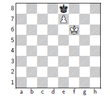
Evaluating Function

position p, include board status, which side to move, history of moves
history -> castling

Perfect evaluating function f(p):
f(p) = 1 for a won position.
f(p) = 0 for a drawn position.
f(p) = -1 for a lost position.
Perfect evaluating function is impossible for most games, and is not fun or educational.

Factors considered in approximate evaluating functions:

• The relative values of differences in materials.
  • The values of queen, rook, bishop, knight and pawn are about 9, 5, 3, 3, and 1, respectively.
  • How to determine good relative values? Static values verse dynamic values?
• Position of pieces
  • Mobility: the freedom to move your pieces.
  • at center , or at corner
  • Doubled rooks
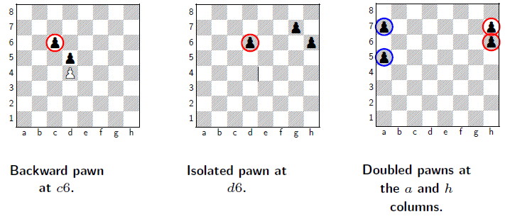
• Pawn structure: the relative positions of the pawns.
  • Backward pawn: a pawn that is behind the pawn of the same color on an adjacent file that cannot advance without losing of itself.
  • Isolated pawn: A pawn that has no friend pawn on the adjacent file.
  • Doubled pawn: two pawns of the same color on the same file
  • these three are all bad pawn
  • Passed pawns: pawns that have no opposing pawns to prevent
  • Pawns on opposite colour squares from bishop.
• King safety.
• Threat and attack.
  • Attacks on pieces which give one player an option of exchanging
  • Pins(小盯大) which mean here immobilizing pins where the pinned piece is of value not greater than the pinning piece
  • Commitments -> 需要保護其他子
• 

Putting "right" coeffcients for diffferent factors
Dynamic setting in practical situations.

evaluating function can be only applied in
relatively quiescent positions.

not in the middle of material exchanging.
not being checked

max-min strategy
In your move, you try to maximize your f(p).
In the opponent's move, he tries to minimize f(p).

A strategy in which all variations are considered out to a
definite number of moves and the move then determined from
a max-min formula is called type A strategy.

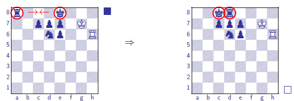
Stalemate
Winning by making the opponent having no legal next move.
suicide move is not legal, and stalemate results in
a draw if it is not currently in check.

Zugzwang(強制被動): In certain positions, a player is at a disadvantage if he is the next player to move.

Programming
- Special rules of games
- Methods of winning
- Basic data structure for positions.
- check for possible legal moves
- Evaluating function.

Forced variations(迫著)
one player has little or no choices in playing

type B strategy
the machine must

1. examine forceful variations out as far as possible and evaluate only at reasonable positions

2. select the variations to be explored by some process

            | 1 if any piece is attacked by a piece of lower value,
   

   g(P) = / or by more pieces then defences of if any check exists
   \ on a square controlled by opponent.
   | 0 otherwise.
   Using this function, variations could be explored until g(P)=0,

effective branching factor is about 2 to 3.
Chinese chess has a larger real branching factor, but its average effective branching factor is also about 2 to 3.

"style" of play by the machine can
be changed very easily by altering some of the coeffcients and
numerical factors involved in the evaluating function

A chess master, on the other hand, has available knowledge of hundreds or perhaps thousands of standard situations, stock
combinations, and common manoeuvres based on pins, forks, discoveries, promotions, etc.
In a given position he recognizes some similarity to a familiar situation and this directs his mental calculations along the lines with greater probability of success.

Need to re-think the goal of writing a computer program that
plays games.
To discover intelligence:
What is considered intelligence for computers may not be considered so for human.
To have fun:
A very strong program may not be a program that gives you the most pleasure.
To Find ways to make computers more helpful to human.
Techniques or (machine) intelligence discovered may be useful to computers performing other tasks

Chap 06 Alpha-Beta Pruning

• standard searching procedure for 2-person perfect-information zero sum games
• terminal position
  • a position whose (win/loss/draw) value can be know

Dewey decimal system

杜威分類法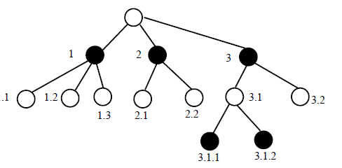

Min-Max method

假設持白子，數字為白子的evaluating function, 在下白子時，取分數最高(max)的，在下黑子時，取分數最低(min)的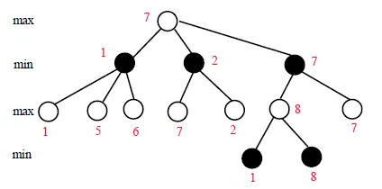

Nega-max method

將下黑子的分數取負號(即為黑子的分數，因為是零和遊戲)
這樣每一層都取最大分數即可

優點是實作較快，程式碼簡潔

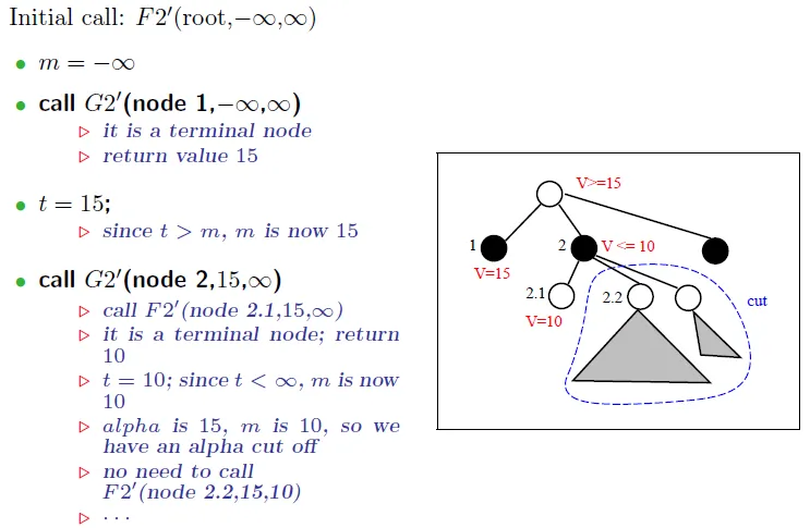
Alpha-Beta cut off

• current search window(score bound) = [α, β]
• If α > β, no need to do further search in current branch
• initial alpha = -∞, beta = ∞

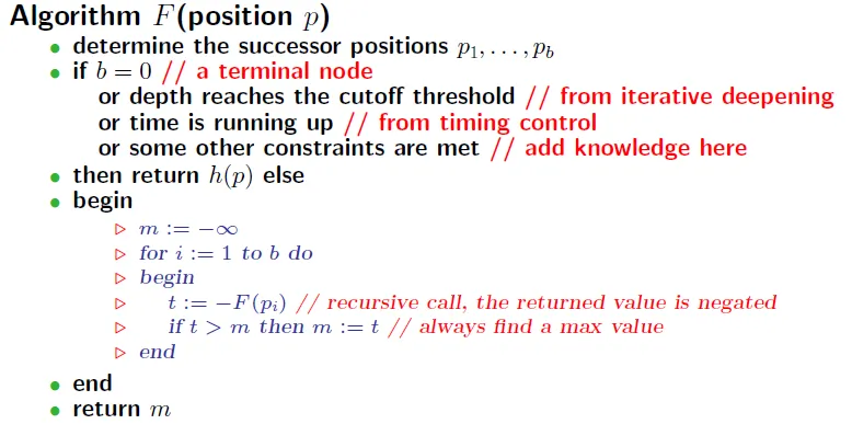
• 只要發現對手有一種反擊方式，使結果比其他手的結果還差，就砍掉這一手(branch)
• 2.1 can cut off 2.x
  • before 2.1 , window = [15, ∞]
  • after 2.1 , window = [15, 10]
• We want to choose the biggest value at root for lower bound, so 2.x is all cut off

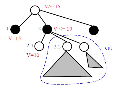
• 只要對手發現自己有一種反擊方式，使結果比其他手的結果還差(α)，就砍掉這一手(branch)
• 1.2.1 can cut off 1.2.x
  • beofre 1.2.1 , 1 bound is [-∞, 10]
  • now 1.2 bound is [15, 10]
• We want to choose smallest value at 1 for upper bound, 1.2.x is all cut off

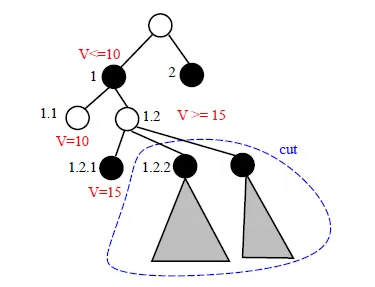
可以砍所有子孫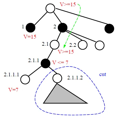

• 2.1.1 is cut off
  • root bound = [15, ∞]
  • 2.1.1 = [-∞, 7]

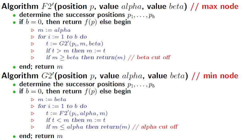
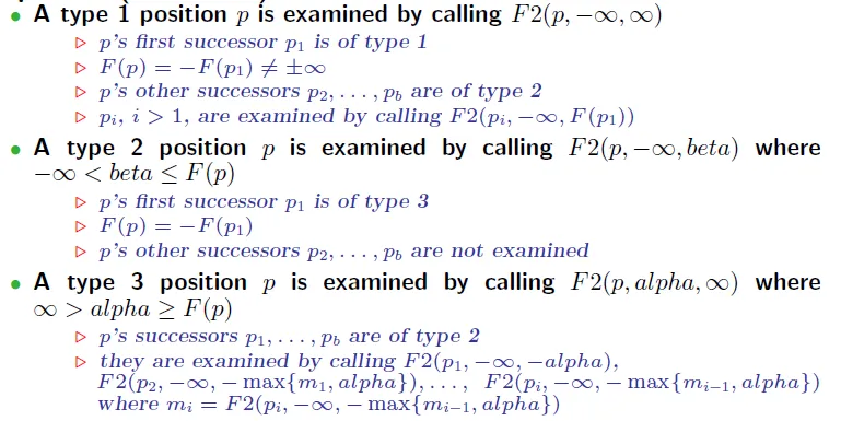
f = white move, find max to be lower bound, do beta cut off
g = black move, find min to be upper bound, do alpha cut off

window變號，回傳的score也要變號
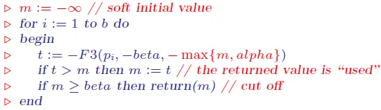
t = -F(pi, -beta, -m)

Analysis for AB pruning

different move orderings give very different cut branches
愈快找到最佳解，可以砍的branch愈多

critical nodes 一定會搜到(cut off之前至少需搜完一個子branch)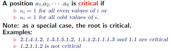

perfect-ordering tree: 每個branch的第一個child就是最佳解
Theorem: 若是perfect-ordering tree, AB pruning 會剛好走過所有 critical nodes
Proof:
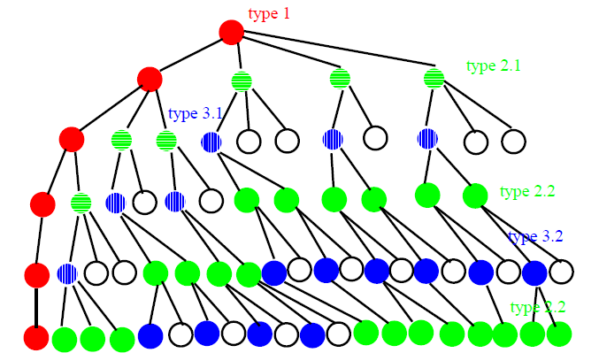
Three Types of critial nodes

• 定義a_i = 第i層的node是第幾個child(杜威分類)
• a_j = 第一個「不是第一個child」的node(如果有的話)
  • a_j-1 = a_j+1 = 1
    • 小於j的node都是1
    • 而且因為是critial node，所以a_j的child一定是1(其他會被砍掉)
• a_l = the last layer

1. root and all node = 1(最左邊, 1, 1.1, 1.1.1 …)
2. l-j = even
   1. j = l (type1 的全部兒子(除了最左邊))
   2. j < l (type3 的全部兒子)
3. l-j = odd
   1. j+1 = l (type2.1 的第一個兒子)
   2. j+1 < l (type2.2的第一個兒子)

We can calculate the least number of nodes to be searched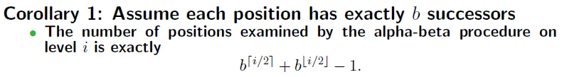

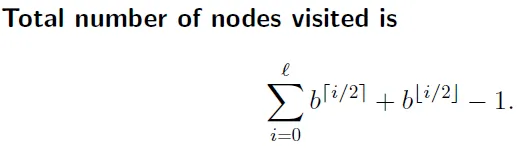
when there're some early terminate nodes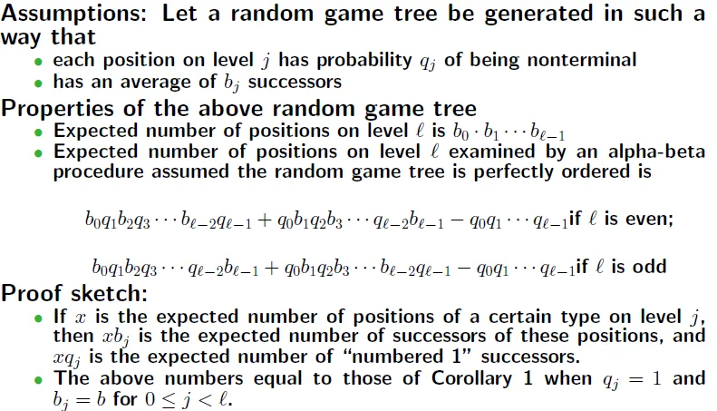
l = even → x.1.x.1... = b0(q1b2)q3...
1.x.1.x... = (q0b1)(q2b3)...(q0b1 = 第一個孩子的全child，若無child，則為(1-qi)*0)

Perfect ordering is not always best when tree are not balanced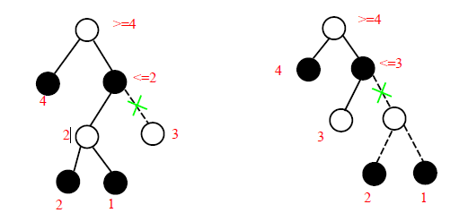
→ When "relative" ordering of children(not perfect order!) are good enough, there are some cut-off

Theorem: 若知道所有的分數，就可以最佳化alpha-beta pruning(計算的點最少，cut最多)
→ 不過如果能算出來就不用search了…

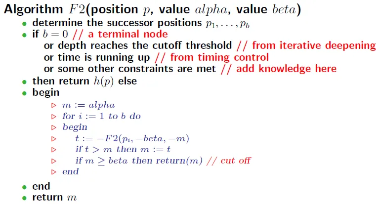
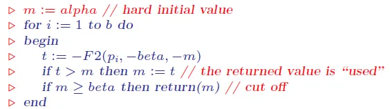
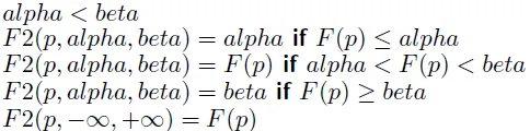
Variations of alpha-beta search

• Fail hard alpha-beta cut(Original) : F2
  • returned value in [α, β]
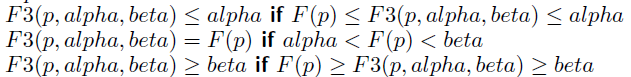
• Fail soft alpha-beta cut(Variation): F3
  • Find "better" value when the value is out of the search window
  • m is the value in this branch(not related to α)
    • use max(m, alpha) to get window
  • return original value m instead of α or β when cut off, which is more precise than fail-hard
  • Failed-high
    • return value > β
  • Failed-low
    • return value < α

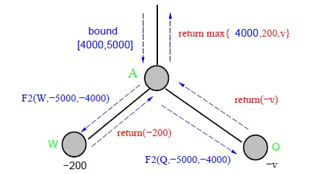
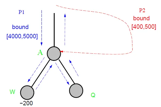
Comparison

• fail-hard
  • return max{4000,200,v}
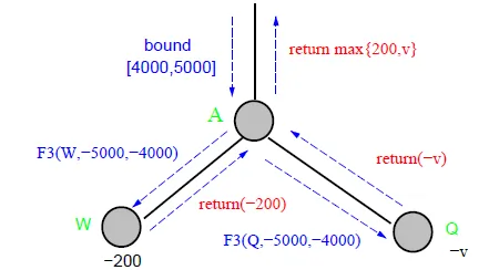
• fail-soft
  • return max{200,v}
• fail-soft provides more information when the true value is out of search window
  • can record better value to be used later when this position is revisited
  • F3 saves about 7% of time than that of F2 when a transposition table is used to save and re-use searched results
  • 記錄F3傳回的值，可減少重複計算的時間，因為下一手的樹在下兩層，大部分node皆相同
    • if p1 is searched, p2 does not need to search again

Questions

• What move ordering is good?
  • search the best possible move first
  • cut off a branch with more nodes first
• What is the effect of using iterative-deepening alpha-beta cut off?
• How about searching game graph instead of game tree?
• Can some nodes be visited more than once?

Pruning Techinique

• Exact algorithms: by mathematical proof
  • Alpha-Beta pruning
  • Scout(in Chap07)
• Approximated heuristics: pruned branches with low probability to be solution
  • in very bad position(盤面太差)
  • a little hope to gain back the advantage(無法逆轉)

Chap07 Scout and Proof Number Search

• Suppose we get at least score s at the First branch
  • want to find whether second branch can get score over s or not

Is there a way to search a tree approximately?

SCOUT

• Invented by Judea Pearl in 1980
• first time: search approximately
  • if there is better value, search again
  • first search can provide useful information in the second search
• TEST whether Tb can return score > v
  • if p is max node → success with only one subbranch > v
  • if p is min node → success with all subbranches > v
  • If success, then search Tb. else, no need to search Tb
• algorithm
  • scout first branch and test other branch
    • if test success, update the value by scout this branch
  • recursive procedure
    • Every ancestor of you may initiate a TEST to visit you
      • will be visited at most d times(= depth)

Time Complexity

• not guarantee(but most of the time) that the visited nodes number are less than alpha-beta
  • may search a branch two times
  • may pay many visits to a node that is cut off by alpha-beta
• TEST: Ω(b^(d/2))
  • but has small argument and will be very small at the best situation
    • if the first subbranch has the best value, then TEST scans the tree fast
    • move ordering is very important
• Comparison
  • alpha-beta
    • cut off comes from bounds of search windows(by ancestors)
  • scout
    • cut off from previous branches' score(by brothers)

Performance

• SCOUT favors "skinny" game trees
  • Show great improvements on depth > 3 for games with small branching factors
  • On depth = 5, it saves over 40% of time
• AB + scout gets average 10~20% improvement than only AB

Null(Zero) window search

• Using alpha-beta search with the window [m,m + 1]
  • result will be failed-high or failed-low
• Failed-high means return value > m + 1
  • Equivalent to TEST(p; m;>) is true
• Failed-low means return value < m
  • Equivalent to TEST(p; m;>) is false
• Using searching window is better than using a single bound in SCOUT

• depth < 3 → no alpha-beta pruning → return value is exact value(no need to search again)
• first-time search → do null window search(scout)
• research → do normal window a-b pruning

Refinements

• Use information from previous search
  • When a subtree is re-searched, restart from the position that the value is returned in first search
• Change move ordering
  • Reorder the moves by priority list

Proof Number Search

binary valued game tree

• 2-player game tree with either 0 or 1 on the leaves

  • and-or tree: min → and, max → or

• most proving node for node u

  • node that if its value is 1, then the value of u is 1

• most disproving node for node u

  • node that if its value is 0, then the value of u is 0

• proof(u): minimum number of nodes to visit to make u = 1

• disproof(u): minimum number of nodes to visit to make u = 0

If value(u) is unknown, then proof(u) is the cost of evaluating u

• If value(u) is 1, then proof(u) = 0
• If value(u) is 0, then proof(u) = ∞
• proof number can be calculate by search childrens
  • disproof number → reverse calculate method of proof number

Usage

• find child u that have min{proof(root); disproof(root)}
• if we try to prove it
  • pick a child with the least proof number for a MAX node
  • pick any node that has a chance to be proved for a MIN node
• if we try to disprove it
  • pick a child with the least disproof number for a MIN node
  • pick any node that has a chance to be disproved for a MAX node
• used in open game tree or an endgame tree because some proof or disproof number is known
  • 1 → proved to win, 0 → proved to lose
  • or used to achieve sub-goal in games

Proof-Number search algorithm

1. keep update number by bottom-up
   1. compare proof number and disproof number of root
2. find the leaf to prove or disprove

Multi-value game tree

• value in [0, 1]
• $proof_v(u)$: the minimum number of leaves needed to visited to make u >= v
  • proof(u) = $proof_1(u)$
• $disproof_v(u)$: the minimum number of leaves needed to visited to make u < v
  • disproof(u) = $disproof_1(u)$
• use binary search to set upper bound of the value

Chap08 Monte-Carlo Game Tree Search

original ideas

Algorithm $MCS_{pure}$

• For each possible next move

  • play this move and then play a lot of random games(play every moves as random)
  • calculate average score

• Choose move with best score

• Original version: GOBBLE in 1993

  • Performance is not good compared to other Go programs(alpha-beta)

• Enhanced versions

  • Adding the idea of minimax tree search
  • Adding more domain knowledge
  • Adding more searching techniques
  • Building theoretical foundations from statistics, and on-line and off-line learning
  • results
    • MoGo
      • Beat a professional human 8 dan(段) with a 8-stone handicap at January 2008
      • Judged to be in a "professional level" for 9 x 9 Go in 2009
    • Zen
      • close to amateur 3-dan in 2011
      • Beat a 9-dan professional master with handicaps at March 17, 2012
        • First game: Five stone handicap and won by 11 points
        • Second game: four stones handicap and won by 20 points

Disadvantage

• average score search != minimax tree search
  • $MCS_{pure}$ prefer right branch, but it's min value is low

First Refinement: Monte-Carlo based tree search

Intuition

• Best First tree growing
  • Expand one level of best leaf(which has largest score)
• if number of simulations is not enough, it can't be a good simulation
  • on a MIN node, if not enough children are probed for enough number of times, you may miss a very bad branch
  • take simulation count into consideration

Second Refinement: UCT

• Effcient sampling

  • Original: equally distributed among all legal moves
  • Biased sampling: sample some moves more often than others

• Observations

  • Some moves are bad and do not need further exploring
    • Need to consider extremely bad luck sitiation
      • e.g. often "randomly" choose bad move and get bad score

• K-arm bandit problem

  • Assume you have K slot machines each with a different payoff, i.e., expected value of returns ui, and an unknown distribution
  • Assume you can bet on the machines N times, what is the best strategy to get the largest returns?

• Ideas

  • Try each machine a few, but enough, times and record their returns
    • For the machines that currently have the best returns, play more often later
    • For the machines that currently return poorly, give them a chance sometimes to check their distributions are really bad or not

UCB: Upper Confidence Bound

• Meaning
  • For a MAX node, Wi is the number of win's for the MAX player
  • For a MIN node, Wi is the number of win's for the MIN player
  • When N is approaching logN, then UCB is nothing but the current winning rate plus a constant
  • When N getting larger, UCB will approachthe real winning rate
• Expand for the move with the highest UCB value
• only compare UCB scores among children of a node
  • It is meaningless to compare scores of nodes that are not siblings
• Using argument c to keep a balance between
  • Exploitation: exploring the best move so far
  • Exploration: exploring other moves to see if they can be proved to be better
• alternative
  • consider the variance of scores in each branch

UCT: Upper Confidence Bound for Tree

• Maintain the UCB value for each node in the game tree
  • Pick path such that each node in this path has a largest UCB score among all of its siblings
  • Pick the leaf node in the path which has been visited more than a certain amount of times to expand

Usable when the "density of goals" is suffciently large

• When there is only a unique goal, Monte-Carlo based simulation may not be useful

new MCT algorithm(with UCT)

Implementation hints

When to use Monte-Carlo

• huge branching number
• cannot easily compute good evaluating function
• Mostly used in Go, Bridge(?)

Rule of Go(圍棋)

• Ko(打劫): 不能有重複盤面
• 可以跳過，不能下自殺步
• Komi: 先手讓子

Implementation

• partition stones into strings(使用共同氣的子) by DFS
• check empty intersection is an eye or not(check neighbors and limits)

Domain independent refinements

Main considerations

• Avoid doing un-needed computations
• Increase the speed of convergence
• Avoid early mis-judgement
• Avoid extreme bad cases

Refinements

• Progressive pruning
  • Cut hopeless nodes early
• All moves at first(AMAF)
  • Increase the speed of convergence
• Node expansion
  • Grow only nodes with a potential
• Temperature
  • Introduce randomness
• Depth-i enhancement
  • With regard to Line 1, the initial phase, exhaustively enumerate all possibilities

Progressive pruning

Each move has a mean value m and a standard deviation σ

• Left expected outcome ml = m - rd * σ

• Right expected outcome mr = m + rd * σ

  • rd is argument

• A move M1 is statistically inferior to another move M2 if M1.mr < M2.ml

• Two moves M1 and M2 are statistically equal if M1.σ < σe and M2.σ < σe and no move is statistically inferior to the other

  • σe is argument which called standard deviation for equality

Remarks

• only compare nodes that are of the same parent
• compare their raw scores not their UCB values
  • If you use UCB scores, then the mean and standard deviation of a move are those calculated only from its un-pruned children
• prune statistically inferior moves after enough number of times of simulation

This process is stopped when

• there is only one move left
• the moves left are statistically equal
• a maximal threshold(like 10000 multiplied by the number of legal moves) of iterations is reached

Two different pruning rules

• Hard: a pruned move cannot be a candidate later on
• Soft: a move pruned at a given time can be a candidate later on if its value is no longer statistically inferior to a currently active move
  • Periodically check whether to reactive it

Arguments

• Selection of rd

  • The greater rd is
  • the less pruned the moves are
  • the better the algorithm performs
  • the slower at each play

• Selection of σe

  • The smaller σe is
  • the fewer equalities there are
  • the better the algorithm performs
  • the slower at each play

• rd plays an important role in the move pruning process

• σe is less sensitive

• Another trick is progressive widening or progressive un-pruning

  • A node is effective if enough simulations are done on it and its values are good

• We can set threshold on whether to expand the best path, for exmaple

  • enough simulations are done
  • score is good enough

All moves at first(AMAF)

• score is used for all moves the same player played in a random game
  • in this example, after simulate r→v→y→u→w, w which has parent v and u which has parent r will be updated, too
• Advantage
  • speeding up the experiments
• Drawback
  • not the same move - move in early game is not equal to late game
  • Recapturing
    • Order of moves is important for certain games(圍棋)
    • Modification: if several moves are played at the same place because of captures, modify the statistics only for the player who played first

Refinement: RAVE

• Let v1(m) be the score of a move m without using AMAF
• Let v2(m) be the score of a move m with AMAF
• Observations
  • v1(m) is good when suffcient number of simulations are starting with m
  • v2(m) is a good guess for the true score of the move m
    • when approaching the end of a game
    • when too few simulations starting with m

Rapid Action Value Estimate (RAVE)

• revised score $v3(m) = a \times v1(m) + (1-a) \times v2(m)$
• can dynamically change a as the game goes
  • For example: a = min{1, Nm/10000}, where Nm is simulation times start from m
    • This means when Nm reaches 10000, then no RAVE is used
  • Works out better than setting a = 0(i.e. pure AMAF)

Node expansion

• May decide to expand potentially good nodes judging from the
  current statistics
• All ends: expand all possible children of a newly added node
• Visit count: delay the expansion of a node until it is visited a certain number of times
• Transition probability: delay the expansion of a node until its \score" or estimated visit count is high comparing to its siblings
• Use the current value, variance and parent's value to derive a good estimation using statistical methods
  Expansion policy with some transition probability is much better than the \all ends" or \pure visit count" policy

Reference

TSHsu講義 2014年版