機器學習技法

尚未寫完

Chap01 SVM

All line is the same using PLA, but WHICH line is best?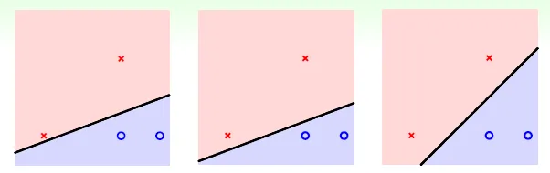
→ 可以容忍的誤差愈大愈好(最近的點與分隔線的距離愈遠愈好)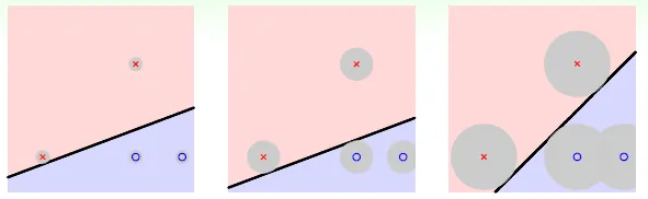
→ fat hyperplane (large margin)(分隔線可以多寬)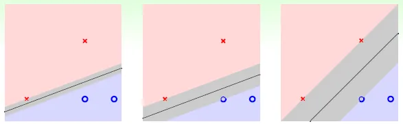

若只有兩個點，必通過兩點連線之中垂線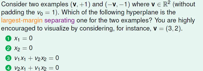

Standard large-margin hyperplane problem

max fatness(w) (max margin)
= min distance($x_n$, w) (n = 1 ~ N)
= min distance($x_n$, b, w) -- (1)
因為 w0 不列入計算(w0 = 常數項參數 = 截距b, x0 必為 1)

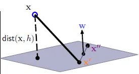
$w^tx$ = 0 → x除去x0成為x' → $w^tx'$ + b = 0
設x', x''都在$w^tx'$ + b = 0平面上，$w^tx'$ = -b, $w^tx''$ = -b → $w^t(x''-x')$ = 0
$w^t$ 垂直於 $w^tx'$ + b = 0平面
distance(x, b, w) = x 到 平面的距離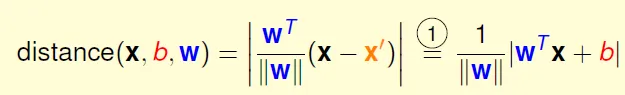

單一data的distance: 因 $y_n(w^t x_n + b) > 0$
$distance(x_n, b, w) = (1/|w|) * y_n(w^t x_n + b)$ -- (2)

specialize
令 $min y_n(w^t x_n + b) = 1$
→ $distance(x_n, b, w) = 1/|w|$
由式子(1),(2)可得 max margin = min distance(x_n, b, w) = 1/|w|
條件為 $min y_n(w^t x_n + b) = 1$

放鬆條件
$y_n(w_t x_n + b) >= 1$ is necessary constraints for $ min y_n(w_t x_n + b) = 1$
if all y_n(w_t x_n + b) > p > 1 -> can generate more optimal answer (b/p, w/p) -> distance 1/|w| is smaller
so y_n(w_t x_n + b) >= 1 → y_n(w_t x_n + b) = 1

max 1/|w| -> min 1/2 * w_t * w

can solve w by solve N inequality

Support Vector Machine(SVM)

只須找最近的點即可算出w
support vector: bounary data(胖線的邊界點)

gradient? : not easy with constraints
but we have:

• (convex) quadratic objective function(b, w)
• linear constraints (b, w)

can use quadratic programming (QP, 二次規劃): easy

Linear Hard-Margin(all wxy > 0) SVM

the same as ‘weight-decay regularization’ within Ein = 0

Restricts Dichotomies(堅持胖的線): if margin < p, no answer
fewer dichotomies -> small VC dim -> better generalization

最大胖度有極限：在圓上，最大 根號3/2

can be good with transform
控制複雜度的方法！
控制複雜度的方法！

Chap02 dual SVM

if d_trans is big, or infinite?(非常複雜的轉換)
find: SVM without dependence of d_trans
去除計算(b, w)與轉換函式複雜度的關係
(QP of d_trans+1 variables -> N variables)

Use lagrange multiplier: Dual SVM: 將lambda視為變數來解


若不符條件，則L()的sigma部分是正的，MaxL()為無限大
若符條件，則L()的sigma部分最大值為0 -> MaxL() = 1/2w^tw
所以Min(MaxL()) = Min(1/2w^tw)

交換max min的位置，可求得原問題的下限

可以得到strong duality(強對偶關係，=)？
若在二次規劃滿足constraint qualification

1. convex
2. feasible(有解)
3. linear constraints

則存在 primal-dual 最佳解(對左右邊均是最佳解)

Dual SVM 最佳解為？

b可以被消除(=0)

w代入得

Karush-Kuhn-Tucker (KKT) conditions

primal-inner -> an = 0 或 1-yn(wtzn+b) = 0(complementary slackness)
=> at optimal all ‘Lagrange terms’ disappear

用KKT求得a(原lambda)之後，即可得原來的(b, w)
w = sigma anynzn
b 僅有邊界(primal feasible)，但b = yn - wtzn when an > 0 (primal-inner，代表必在SVM邊界上)

重訂support vector的條件(a_n >0)

=> b, w 都可以只用SV求到

SVM:找到有用的點(SV)

Standard hard-margin SVM dual

經過整理

現在有N個a, 並有N+1個條件了

when N is big, qn,m is dense array and very big(N >30000, use >3G ram)
use special QP solver

SVM 和 PLA 比較

w = linear combination of data => w represented by data
SVM: represent w by only SV

Primal: 對(b,w)做特別縮放
Dual: 找到SV 和其 lagrange multiplier

問題：q_n,m 需要做O(d_trans)的運算，如何避免？

Chap03 Kernel SVM

(z_n^T)(z_m)如何算更快

轉換+內積 -> Kernel function

use O(d) instead of O(d^2)

用kernel簡化！(gsvm -> 無w)

Kernel Hard-Margin SVM

polynomial Kernel

簡化的kernel: 對應到同等大小，不同幾何特性(如內積)的空間

r影響SV的選擇

可以快速做高次轉換(和二次相同複雜度)

特例: linear只需用 K1 = (0+1xtx)^1

infinite Kernel

taylor展開

無限維度的Gaussian Kernel (Radial Basis Funtion(RBF))

large => sharp Gaussians => ‘overfit’?

Kernel選擇

linear kernel: 等於沒有轉換，linear first, 計算快
polynomial: 轉換過，限制小，strong physical control, 維度太大K會趨向極端值
-> 平常只用不大的維度
infinite dimension:
most powerful
less numerical difficulty than poly(僅兩次式)
one parameter only
cons: mysterious -- no w , and too powerful

define new kernel is hard:
Mercer's condition:

Chap04 Soft-Margin SVM

overfit reason: transform & hard-margin(全分開)

Soft-Margin -- 容忍錯誤，有錯誤penalty，只有對的需要符合條件

缺點：
No QP anymore
error大小:離fat boundary的距離

改良：求最小(犯錯的點與boundary的距離和)(linear constraint, can use QP)

parameter C: large when want less violate margin
small when want large margin, tolerate some violation

Soft-margin Dual: 將條件加入min中

化簡後得到和dual svm相同的式子(不同條件)

C is exactly the upper bound of an

Kernel Soft Margin SVM

more flexible: always solvable

(3)->solve b:
若as < C(unbounded, free), 則b的求法和hard-margin一樣

但soft-margin還是會overfit...

physical meaning

not SV(an = 0): C-an != 0 -> En = 0
unbounded SV(0 < an < C，口) -> En = 0 -> on fat boundary
bounded SV(an = C, △) -> En >= 0(有違反，不在boundary上)
-> 只有bounded SV才可違反

difficult to optimize(C, r)

SVM validation

leave-one-out error <= #SV/N
若移除non-SV的點，則得出的g不變
-> 可以靠此特性做參數選擇(不選#SV太大的)

Chap05 Kernel Logistic SVM

實用library: linear:LIBLINEAR nonlinear:LIBSVM

將E替代 -> 像是 L2 regularization

缺點：不能QP, 不能微分(難解)

large margin <=> fewer choices <=> L2 regularization of short w
soft margin <=> special err
larger C(in soft-margin or in regularization) <=> smaller lagrange multiplier <=> less regularization

We can extend SVM to other learning models!

look (wtzn + b) as linear score(f(x) in PLA)

we can have Err_svm is upper bound of Err0/1
(hinge error measure)

Err_sce: 與svm相似的一個logistic regression

L2 logistic regression is similar to SVM,
所以SVM可以用來approximate Logistic regression?
-> SVM當作Log regression的起始點? 沒有比較快(SVM優點)
-> 將SVM答案當作Log的近似解(return theta(wx + b))? 沒有log reg的意義(maximum likelyhood)
=> 加兩個自由度，return theta(A*(wx+b) + B)
-> often A > 0(同方向), B~=0(無位移)

將原本的SVM視為一種轉換

Platt's Model

kernel SVM在Z空間的解 -- 用Log Reg微調後 --> 用來近似Log Reg在Z空間的解(並不是在z空間最好的解)

solve LogReg to get(A, B)

能使用kernel的關鍵：w為z的線性組合

Representer Theorem: 若解L2-正規化問題，最佳w必為z的線性組合
將w分為(與z垂直)+(與z平行), 希望w_垂直 = 0
證：(原本的w) 和 (與z平行的w) 所得的err是一樣的(因為w_垂直 * z = 0)
且w平行比較短
所以min w 必(與z平行)

結果：L2的linear model都可以用kernel解！

將w = sum(B*z) = sum(B*Kernel)代入logistic regression
-> 解B

Kernel Logistic Regression(KLR)
= linear model of B

把 kernel當作轉換, kernel當作regularizer
= linear model of w
with embedded-in-kernel transform & L2 regularizer
把 kernel內部(z)當作轉換(?), L2-regularizer

警告：算出的B不會有很多零

soft margin SVM ~= L2 LOG REG, special error measure:hinge
在z空間解log reg -> 用representor theorem 轉換為一般log reg, 有代價

Chap 06 Support Vector Regression(SVR)

ridge regression : 有regularized的regression
如何加入kernel?

Kernel Ridge Regression

用representor theorem代入後得到regularization term 和 regression term

因為kernal必為為psd，所以B必有解 O(N^3)

g(x) = wz = sum(bz)z = sum(bk)

與linear的比較：
kernel自由度高
linear為O(d^3+d^2N)
kernel和資料量有關，為O(N^3)，檔案大時不快

LS(least-squares)SVM = kernel ridge regression:
和一般regression boundary差不多，但SV很多(B dense)
=> 代表計算時間長
=> 找一個sparse B?

tube regression:

insensitive error:容忍一小段的差距(在誤差內err = 0，若超過, err只算超過的部分)
error增加的速度變慢

學SVM，解QP, 用DUAL, KKT->sparse

regulizer 和 超過tube上界的值，超過tube下界的值

參數：C(violation重視程度), tube範圍

作dual: lagrange multiplier + KKT condition

在tube裡面的點：B=0
=> 只要tube夠寬，B為sparse

Linear, SVM Summary

first row: less used due to worse performance
third row: less used due to dense B
fourth row: popular in LIBSVM

Chap07 Blending and Bagging

Selection: rely on only once hypothesis
Aggregation: mix or combine hypothesiss
select trust-worthy from their usual performance
=> validation
mix the prediction => vote with different weight of ballot
combine predictions conditionally(when some situation, give more ballots to friend t)

Aggregation可做到：

1. feature transform(?), 將hypothesis變強
2. regularization(?)
   控制 油門 和 煞車
   

uniform blending: 一種model一票，取平均
證明可以比原本的Eout小:

一個演算法A的表現，可以用其hypothesis set中的"共識"來表示，等於共識的表現，加上共識的變異數，uniform blending就是將某些在A的hypothesis取平均(變成新的演算法A')來減少A'的變異數
expected performance of A = expected deviation to consensus + performance of consensus

linear blending: 加權(線性)平均，權重>0

求類似linear regression的式子: 兩段式學習，先算出許多g，再做 linear regression -> 得到答案G
限制：權重a>0 -> 將error rate大的model反過來用(error rate = 99%, 取其相反答案即可將error rate = 1%)

any blending(stacking): 可用non-linear model(???)

算出g1-, g2- ...   
phi-1 = (g1-, g2-, ...)   
transform validation data to Z = (phi-1(x), y)   
compuate g = AnyModel(Z, Y)   
return G = g(phi(x))
phi = (g1, g2 ... )

比較：linear blending

compuate a = AnyModel(Z, Y)   
return G = a * phi(x)

learning: 邊學邊合，

bootstrapping: 從有限的資料模擬出新的資料
bootstrap data: 從原本資料選擇N筆資料(可重複)
Virtual aggregation
bootstrap aggregation(bagging): 由bootstrap data訓練g，而非原資料
-> meta algorithm for [base algorithm(可使用不同演算法)]

Chap08 Adaptive Boosting

教小學生辨認蘋果:
由一個演算法提供[會混淆的資料]
由其他hypothesis提出一個不同的小規則來區分

給不同的data權重，會混淆的占較大比例，取min Ein = avg(Wn * err(xn, yn))，可用SVM, lin_reg, log_reg解Wn

gt = argmin(sum(ut * err))
gt+1 = argmin(sum(ut+1 * err))

找完gt後，gt+1應該要找和gt不相似的->找ut+1使gt的err rate接近0.5(隨機)。

err rate = 錯誤資料權重和 / (錯誤資料權重和 + 正確資料權重和) = 1/2
=> 希望 正確資料權重和 = 錯誤資料權重和
在gt中正確的資料, 權重要乘(err rate)
在gt中錯誤的資料, 權重要乘(1-err rate)
如此一來兩者之和將會相等

若scale factor = S = sqrt((1-err rate) / err rate)
incorrect *= S
correct *= 1/S
若 S>1:
→ err rate <= 1/2
→ incorrect↑, correct↓, close to 1/2

u1 可設所有為1/N，得到min Ein
G 設uniform會使成績變差

Adaptive Boosting(皮匠法)

邊做邊算at

希望愈好的gt，at愈大
-> 設at = ln(St) (S = scale)
if(err rate == 1/2) -> St = 1 -> at = 0
if(err rate == 0) -> St = inf -> at = inf

只要err rate < 1/2 , 就可以參與投票：群眾的力量

adapative boosting 的 algorithm 選擇(不需強演算法):
decision stump: 三個參數：which feature, threshold(線), direction(ox)，可以使Ein <= 1/2

Chap09 Decision Tree

Traditional learning model that realize conditional aggregation
模仿人類決策過程

Path View:
G = sum(q * g)
q = condition (is x on this path?)
g = base hypothesis, only constant, leaf in tree

Recursive View:
G(x) = sum([b(x) == c] * Gc(x))
G: full tree
b: branching criteria
Gc: sub-tree hypothesis

advantage: human-explainable, simple, efficient, missing feature handle, categorical features easily, multiclass easily
disadvantage: heuristic, little theoretical
Ex. C&RT, C4.5, J48...

four choices: number of branches, branching
criteria, termination criteria, & base hypothesis

C&RT(Classification and Regression Tree):
Tree which is fully-grown with constant leaves
C = 2(binary tree)，可用decision stump
gt(x) = 在此分類下output最有可能(出現最多次的yn or yn平均)
-> 分得愈純愈好(同一類的output皆相同)

impurity = 變異數 or 出現最多次的yn的比率

popular to use :
Gini for classification
regression error for regression

terminate criteria:

1. all yn is the same: impurity = 0
2. all xn the same: cannot cut

if all xn different: Ein = 0
low-level tree built with small D -> overfit

regularizer: number of leaves
argmin(Ein(G) + c * number of leaves(G))
實作：一次剪一片葉子，選最好的

相較數字的feature, 處理類型問題較簡單

Surrogate(代理) branch:
找一些與最好切法相近的，若data features missing, 則使用之

與adaboost相比：片段切割，只在自身subtree切

Chap10 Random Forest

Random Forest = bagging + fully-grown random-subspace random-combination C&RT decision tree

highly parallel, 減少 decision tree的variance

增加decision tree diversity

1. random sample features from x(random subspace of X)
   -> efficient, can be used for any learning models
   10000個features, 只用100個維度來learn

2. 將 x 作 低維度random projection -> 產生新的feature(斜線切割), random combination

Out-of-bag

out-of-bag: not sampled after N drawings
N個data抽N次，沒被抽到機率 ~= 1/e
=> 將沒抽到的DATA作g的validation(通常不做，因為g只為G的其中之一)
=> 將沒抽到的DATA作G的validation，Eoob = sum(err(G-(xn))) (G-不包含用到xn的g)

Eoob: self-validation

Feature Selection

want to remove redundant, irrelevant features...

learn a subset-transform for the final hypothesis

advantage: interpretability, remove 'feature noise', efficient
disadvantage: total computation time increase, 'select feature overfit', mis-interpretability(過度解釋)

decision tree: built-in feature selection

idea: rate importance of every features
linear model: 看w的大小
non-linear model: not easy to estimate

idea: random test
put some random value into feature, check performance↓，下降愈多代表愈重要

random value

• by original P(X = x)
• bootstrap, permutation

performance: 算很久
importance(i) = Eoob(G, D) - Eoob(G, Dp) (Dp = data with permutation in xn_i)

strength-correlation decomposition
s = average voting margin(投票最多-投票第二多...) with G
p = gt之間的相似度
bias-variance decomposition

Chap11 Gradient Boost Decision Tree

Chap12 Neural Network