人工智慧

發表於 2015-02-25 分類於筆記文章字數： 38k

Introduction

What is AI? → What is definition of Intelligence?

Artificial Intelligence(A.I.) or WALL.E
human-like or robot with intelligence
there are various defintion of AI
goal of AI : To create intelligent machines

Multiple Dimensions of Intelligence(多元智能)
- Linguistic(語言), Logico-mathematical, Spatial, Musical, Kinesthetic(動作), Intrapersonal, Interpersonal
Intelligent Behavior
- The ability to solve complex problems
- Learning from experience
- Adaptability(適應性)
- Self-awareness(自我意識)
- Dealing with incomplete information
- Action under time pressure
- Creativity
- Common sense reasoning etc. (really hard to teach computer)
Fundamental Elements of Intelligence
- Prediction – Imagining how things might turn out rather than having to try them explicitly
- Response to change – Responding with intelligent action instead of inalterable instinct or conditional reflexes
- Intentional action – Having a goal and selecting actions appropriate to achieving the goal
- Reasoning – starting with some collection of facts and adding to it by any inference method

Turing Test

"Can machines behave intelligently?"
now it is not criteria of AI(You can use database or some way to "cheat")

Alan Turing (1912-1954)

1936: The Turing machine, computability, universal machine
1950: The Turing Test for machine intelligence

Taxonomy of AI

AI classess

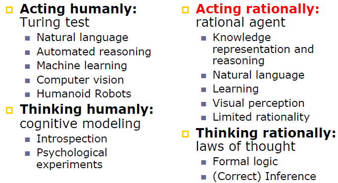
Acting rationally

do the right thing
- be expected to maximize goal achievement, given the available(limited) information
Doesn't necessarily involve thinking
- blinking reflex

The History of AI

The gestation of AI (1943-1956)
Dartmouth conference (Summer of 1956)
- Participants: McCarthy, Minsky, Shannon, Rochester, More(Princeton), Newell, Simon (CMU), Solomonoff, Selfridge(MIT), Samuel (IBM)
- "AI" first be named
Early enthusiasm and expectations (1952-1969)
A dose of reality (1966-1974)
Shakey the Robot (1966-1972)
- the first mobile robot to reason about its actions
  - can do perception, world-modeling, and acting
- often shakes
Knowledge-based systems (1969-1979)
AI (expert systems) becomes an industry (1980-1988)
The return of neural networks (1986-1995)
Broader technical development: probability, ALife, GA, soft computing (1988-)
Machine learning and data mining (1990- )
Intelligent agents (1995- )
Bayesian probabilistic reasoning

Historical Achievements

Deep Blue defeated the reigning world chess champion Garry Kasparov in 1997
Proved a mathematical conjecture (Robbins conjecture)unsolved for decades
No hands across America (driving autonomously 98% of the time from Pittsburgh to San Diego)
- Autonomous Land Vehicle In a Neural Network(ALVINN)
  - a perception system which learns to control the NAVLAB vehicles by watching a person drive.
During the 1991 Gulf War, US forces deployed an AI logistics planning and scheduling program that involved up to 50,000 vehicles, cargo, and people
NASA's on-board autonomous planning program controlled the scheduling of operations for a spacecraft
- Mars: Spirit, Opportunity
Proverb solves crossword puzzles better than most humans
Stanley drove 132 miles to win the Grand Challenge
- DARPA(美國國防遠景研究規劃局) give 1 million in 2004
- investment in competition is far better than in research of university

Other Usage of AI

on market
- floor-cleaning
for fun
- soccer
- pet
human-like
- QRIO(sony)
- Asimo(Honda)
in art: "Aaron"
- Inspired by the scribbling behavior of young children
  - construction of simple core-figures
  - a simple strategy for tracing a path around them
- Online auction for > $2000 a piece

Chap02 Agents

agent

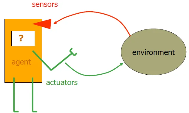
take information from environment through sensors
do reaction that would probably change the environment through actuators
Human agent
- Sensors: eyes, ears, and other organs
- Actuators: hands, legs, mouth, and other body parts

Agents and environments

"do the right thing" is the one that will cause the agent to be most successful

Performance measure
- An objective criterion for success of an agent's behavior
- affects what agent behaves
agent function
- agent (function) = architecture + program
- in order to maximize the performance

Rationality

Rationality is distinct from omniscience (all knowing with infinite knowledge，全知)
Rationality is distinct from clairvoyant(know every information)
- Action outcomes may not be as expected
Rationality is exploration, learning, autonomy(自治)
- perform actions to obtain useful information
- learn and adapt
- actions are determined by its own experience

Task Environment: PEAS

High-Level Descriptions of AI Agents
- Including Performance measure, Environment, Actuators, Sensors
specify the setting for intelligent agent design

Ex. CubeStormer3, which is a rubik cube solver:

Performance measure: Time(= number of steps that agent uses), correctness
Environment: different patterns of rubik cube
Actuators: various robotic arms, smart phone screen
Sensors: camera

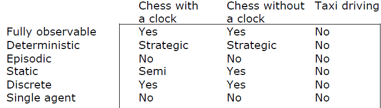
Environment types

Fully observable (vs. partially observable): Sensors can access all environment at each point in time

Deterministic (vs. stochastic): next environment is completely determined by the current state and agent's action
If next environment is determined by actions of all agents, it's called strategic(戰略的)

Episodic (vs. sequential): choice of action in each episode depends only on the episode itself
Sequential environments require memory of past actions to determine the next best action. Episodic environments are a series of one-shot actions

Static (vs. dynamic): The environment is unchanged while agent is thinking
The environment is semi-dynamic if the environment itself does not change with the passage of time but the agent's performance score does
Ex. Taxi driver: Dynamic, Image analysis: Semi

Discrete (vs. continuous): A limited number of distinct, clearly defined perception area
Ex. Driving: continuous, chess games: discrete

Single agent (vs. multi-agent): An agent operating by itself in an environment

The real world is partially observable, stochastic, sequential, dynamic, continuous, multi-agent

chess and taxi environment

Agent types

Table-Lookup Agent(reflex agent)
- has many drawbacks
- huge table
- time-wasting to build the table
- no autonomy
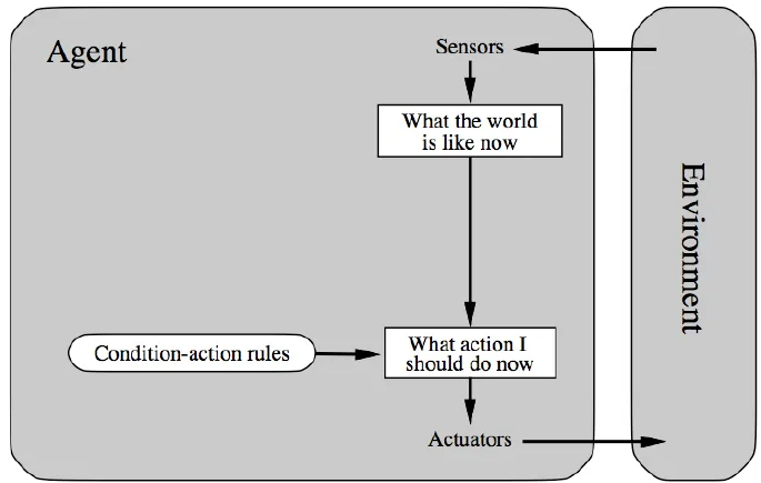
Condition-Action Agent
- four types(generality from low to high)
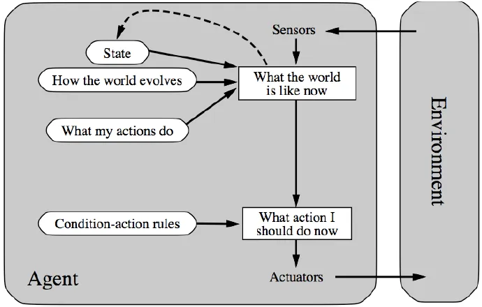
- Simple reflex agents
  - Always Infinite Loop
- Model-based reflex agents
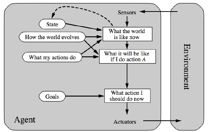
  - Know how world evolves
- Goal-based agents
  - use knowledge about goal to achieve it
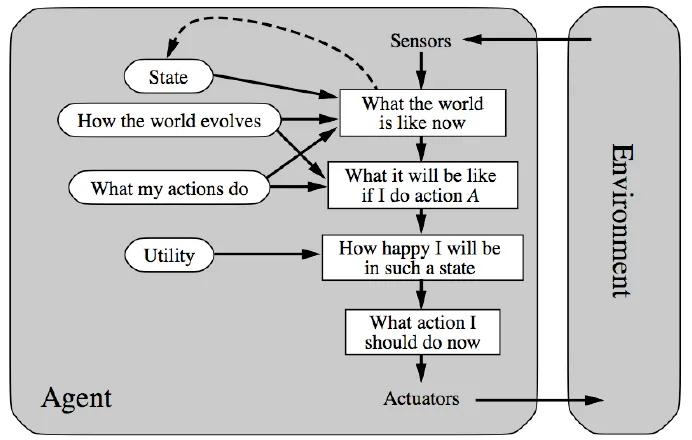
- Utility-based agents
  - utility: value of happiness
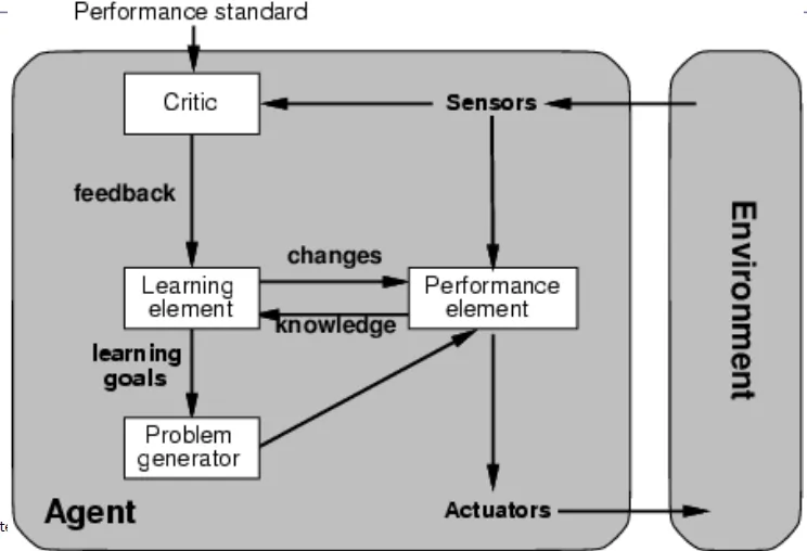
Learning agents
- learning element modifies performance element base on feedback of critic
  - critic: how the agent is doing
  - performance element select proper action
- Problem generator
  - Tries to solve the problem differently instead of optimizing
- Example
  - Knowledge Navigator (Apple, 1987)
  - IBM Watson

Chap03 Search

Search is a universal problem solving mechanism that

Systematically explores the alternatives
Finds the sequence of steps toward a solution
Search in a problem space is claimed to be a completely general model of intelligence
problem space: area that needs to be examined to solve a problem
- the number of the leaf nodes in search tree when there is solution
state space: the set of values which a process can take
- the number of the legal positions in a game

Problem-solving agents

/* s is sequence of actions */
repeat {
	percept = observeWorld();
	state = updateState(state, p);
	if s is empty then {
		goal = formulateGoal(state);
		prob = formulateProblem(state, goal);
		s = search(prob);
	}
	action = first(s);
	s = remainder(s);
}
until false; /* i.e., forever */

Formulate goal → Formulate problem(state, action) → Find solution by search

Problem types

single-state problem
- Deterministic, fully observable
sensorless problem
- Non-observable
contingency(可能性) problem
- Nondeterministic and/or partially observable
- percepts provide new information about current state
exploration problem
- Unknown state space

Problem formulation

A problem is defined by four items

initial state
actions or successor function
goal test function
path cost (optional)

A solution is a sequence of actions from initial state to goal state

Problem Domains

Real-world problems

Route-finding
Touring: travelling
- salesperson problem
VLSI layout
Automatic assembly sequencing
Scheduling & planning
Protein design

Implementation: States vs. Nodes

A state is physical configuration(座標，位置，盤面)
A node is a data structure constituting part of a search tree
- includes state, parent node, action, path cost g(x), depth

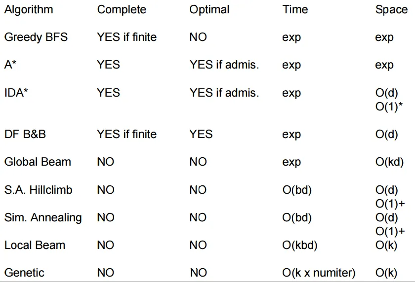
Search Property

Strategies are evaluated by

completeness: does it always find a solution if one exists?
time complexity: number of nodes generated
space complexity: maximum number of nodes in memory
optimality: does it always find a least-cost solution?

Type of Search

可參考電腦對局理論，兩者的complexity算法不同

use only the information available in the problem definition

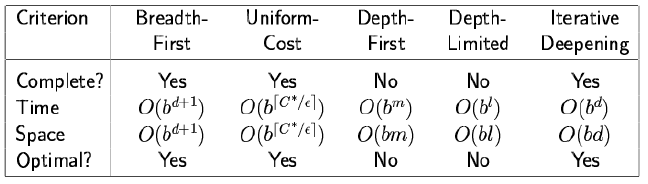
Breadth-first search
- Expand shallowest unexpanded node
- fringe is a queue
Uniform-cost search
- used when "cost != depth"
- Expand least cost(g(n), cost from start to this node) unexpanded node
- Time Complexity: # of nodes with g ≤ cost of optimal solution
  - $O(b^{ceiling(\frac{C*}{ε})})$
  - C* is the cost of the optimal solution
  - ε is small constant
  - How does it compare with $b^d$?
Depth-first search
- Expand deepest unexpanded node
- frontier is a stack
- not complete when there are loops or there are infinite nodes
Depth-limited search
- Preferred uninformed search method
- Iterative deepening search
  - uses only linear space
  - take a little more time

Graph Search

Graph Search vs. Tree Search

Graph Search always need to record closed list to prevent loop
Dijkstra’s Shortest Path Algorithm
- find the shortest path between each pair of nodes
- Order nodes in priority queue to minimize actual distance from the start
- Generalizes BFS that edges can have different lengths/weights

Chap03b Informed Search

Best-First Search

use evaluation function f(n) for each node
Expand most desirable(lowest cost in total) unexpanded node
Order nodes in priority queue to minimize estimated distance to the goal = h(n)
Special cases
- greedy best-first search
  - expands the node that appears to be closest to goal
- A* search
Property
- Complete? No – can get stuck in loops
- Time? O(bm), but a good heuristic can give a lot of improvement
- Space? O(bm) -- keeps all nodes in memory
- Optimal? No
- visits far fewer nodes, but may not provide optimal solution

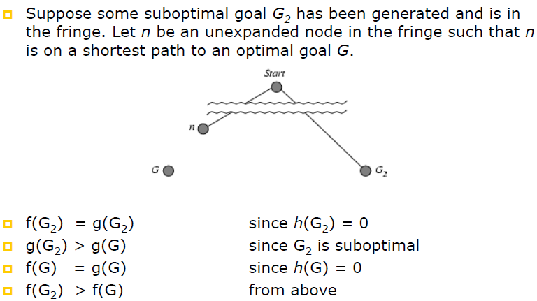
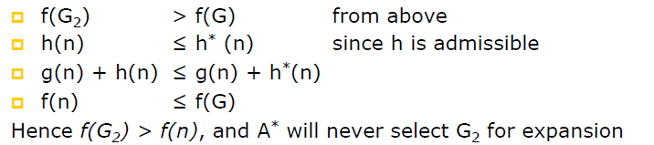
A* Search

avoid expanding paths that are already expensive
Evaluation function f(n) = g(n) + h(n)
- f(n) = estimated total cost of path through n to goal
- g(n) = cost so far to reach n
- h(n) = estimated cost from n to goal
- expands nodes in order of increasing f value
Theorem: If h(n) is admissible, A using TREESEARCH is optimal*
- proof :
Theorem: The search space of A grows exponentially unless the error in the heuristic function(real cost from n to goal - h(n)) grows no faster than the logarithm of the actual path cost*
Property
- Complete? Yes (unless there are infinitely many nodes with f ≤ f(G) )
- Time? Exponential
- Space? Keeps all nodes in memory
- Optimal? Yes
- Efficient? A* is optimally efficient for any heuristic function
  - no other optimal algorithm is guaranteed to expand fewer nodes than A*

Iterative deepening A*(IDAstar)

Cutoff by f-cost
- upper bound of f(n)
- If don't find solution
  - Increase the bound to
  - the minimum of the f-values that exceeded the previous bound
?? Not suitable for real-valued costs
Advantage: Linear space

Recursive best-first search(RBFS)

only keep track of total cost of the best alternative path
if best node exceeds alternative f(n)
- unwinds back to the alternative path
Back up value of dropped node to its parent
- if all other paths are worse than it, we should use it again
Advantage: Linear space

disadvantage of IDA* and RBFS

not good for graphs
- can’t check for repeated states other than those on current path
use too little memory
- can't use full memory

Simplified Memory-bounded A*(SMA star)

Expand the best leaf until memory is full
When memory full
- Drop the worst(highest f-value) leaf node
Back up value of dropped node to its parent
Property
- use full of the memory usage
- complete when meory is enough to store the shallowest solution
- optimal when meory is enough to store the shallowest optimal solution

A heuristic is consistent if for every node n, f(n) is non-decreasing along all paths
Theorem: If h(n) is consistent, A using GRAPHSEARCH is optimal*
(every consistent function is admissible)

Inventing Better Heuristic Functions

quality of heuristic: effective branching factor b*
If h2(n) ≥ h1(n) for all n (both admissible), then h2 dominates h1(far better than)

Relaxed problems
- problem with fewer restrictions
  - admissible and consistent
    - exact cost of problem → consistent
- Original: move any tile to adjacent empty squares
  - Relaxed: Move from A to B, if A is adjacent to B → Manhattan distance
  - Relaxed: Move from A to B, if B is empty → Gaschnig’s heuristic (1979)
Composite heuristics
- h(n) = max (h1(n),…,hm(n))
Weighted evaluation function
- fw(n) = (1-w)g(n) + w h(n)
Linear combination of features
- h(n) = c1x1(n) + … + ckxk(n)
- no assure admissible or consistent
Statistical information
Search cost
- Good heuristic function should be computed efficiently
Sub-Problems
- solution cost of a sub-problem of a given problem
Example
- Linear Conflict Heuristic
  - Given two tiles in their goal row, but reversed in position, additional vertical moves can be added to Manhattan distance

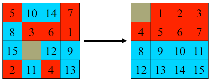
Adding Pattern Database Heuristics

pattern database
- store exact solution costs of subproblems
How to make sure heuristic function can add with admissible? → do not affect each other
- disjoint pattern database
The 7-tile database contains 58 million entries
- 20 moves needed to solve red tiles
The 8-tile database contains 519 million entries
- 25 moves needed to solve blue tiles
Overall heuristic is 20+25=45 moves
On 15 puzzle, IDA* with pattern database heuristics is about 10 times faster than with Manhattan distance(Culberson and Schaeffer, 1996)
can also be applied to Rubik’s Cube

Summary: all informed algorithms

Chap04 Beyond Classical Search

Local Search Algorithms

Used when the path to the goal does not matter

State space: the set of all states reachable from initial state

local search algorithms

iterative improvement
- keep a single "current" state and try to improve it
advantage
- use constant space
- useful to solve optimization problems(最佳化問題)

Example

Traveling Salesperson Problem
- use 1% additional cost than optimal solution
- solved very quickly with thousands of cities
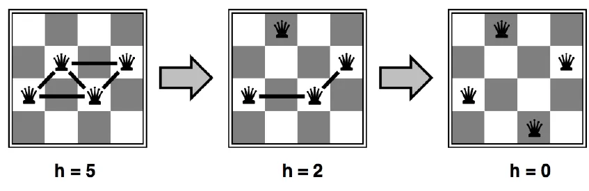
N-queen problem
- can solve N = 1000000 quickly
Widely used in VLSI layout, airline scheduling, etc

Three algorithms

hill climbing
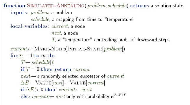
simulated annealing
genetic algorithms

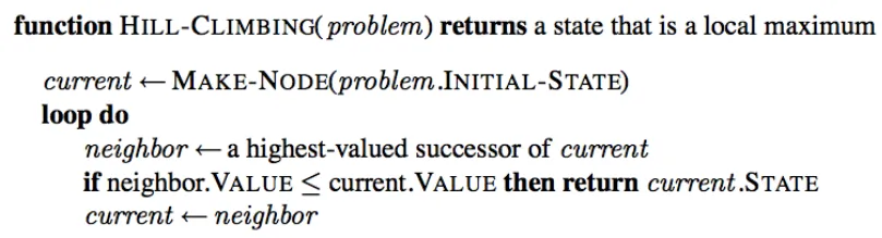
Hill climbing(爬山)

greedy local search
- grab the best neighbor as successor
若所有鄰居的值都比現值小，則認為現值是最大值
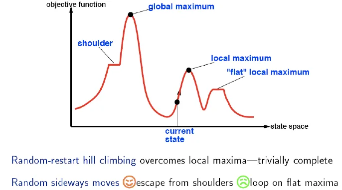
可能會走到Local maxima
走到平地的時候
- 限制走平地的步數

變形

Stochastic hill-climbing
- choose uphill moves by 斜度 as probability
First-Choice hill-climbing
- generating successor until it is better than parent
Random-restart hill-climbing
- random generate initial state until goal is found

Simulated annealing

escape local maxima
- allowing some "bad" moves
- gradually decrease their frequency & size
- this probability reach Boltzman distribution
  - If T decreases slowly enough, then simulated annealing search will find a global optimum with probability approaching

Local Beam Search

Keep track of (top) k states rather than just one
useful information is passed among all parallel search threads
Problem: all k states possibly end up on same local hill
- Stochastic Local Beam Search
  - choose k successors randomly, biased towards good ones(successor that has better score has more probability to be choosed)

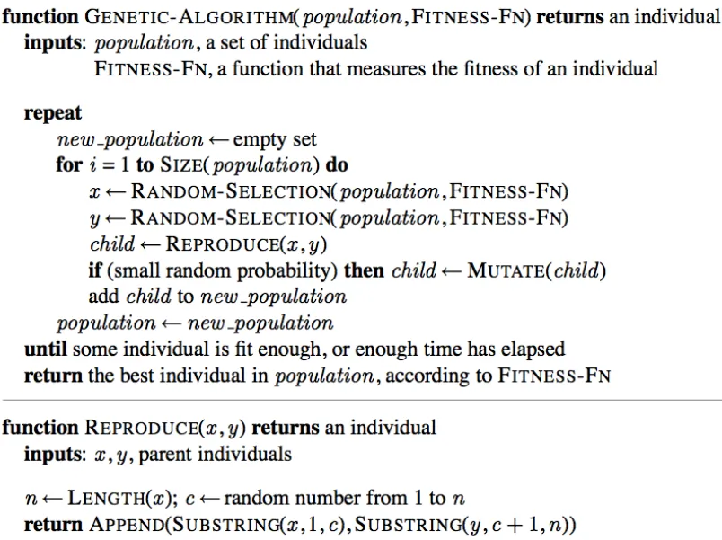
Genetic algorithms

Stochastic local beam search + generate successors from pairs
Population
- Start with k randomly individuals
Individual(state)
- represented as a string by finite symbols (often a string of 0s and 1s)
- substring must be meaningful
Fitness function: evaluation of the “goodness” of a given state
- N-queen: number of non-attacking queens pairs (min = 0, max = 8 × 7 / 2 = 28)
Produce successors
- selection, crossover(交配, combine two parents), and mutation(突變)
Schema
- 8-Queen: 2468xxxx → 24681357, 24681753 ...
- if average fitness value of schema is better than mean, instances of schema will grow

Local search in continuous spaces

Most of real-world environments are continuous
Example: Airport Site Planning
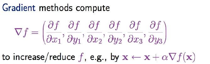
- 6-D state space (x1,y1),(x2,y2),(x3,y3)
- Objective function f(x1,y1,x2,y2,x3,y3) = sum of squared distances from each city to its nearest airport
Successor function would return infinitely many states
- Solution
  - Discretization(離散化)
  - Gradient of the objective function
    - Empirical(經驗主義) gradient
      - take a little change in each coordinate to fit discretization
    - Line search
      - repeatly double the size of updating until the value descrease(下坡)
  - Newton-Raphson method
    - solve ∇f(x) = 0

Searching with nondeterministic actions

solution is not sequence, but a contingency plan(strategy)
Unreliable Vacuum World
- sometimes can not action will fail
Solutions(nested if-then-else statements)
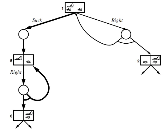
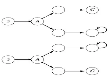
- AND-OR Search Tree
  - P if ((Q&R) | S)
  - Q if (T | U)
  - and → environment's choice(fail or not)
  - or → your own choice
- returns a set of possible outcome states
Ex. Slippery Vacuum World
- Movement actions sometimes fail
- use cyclic plans

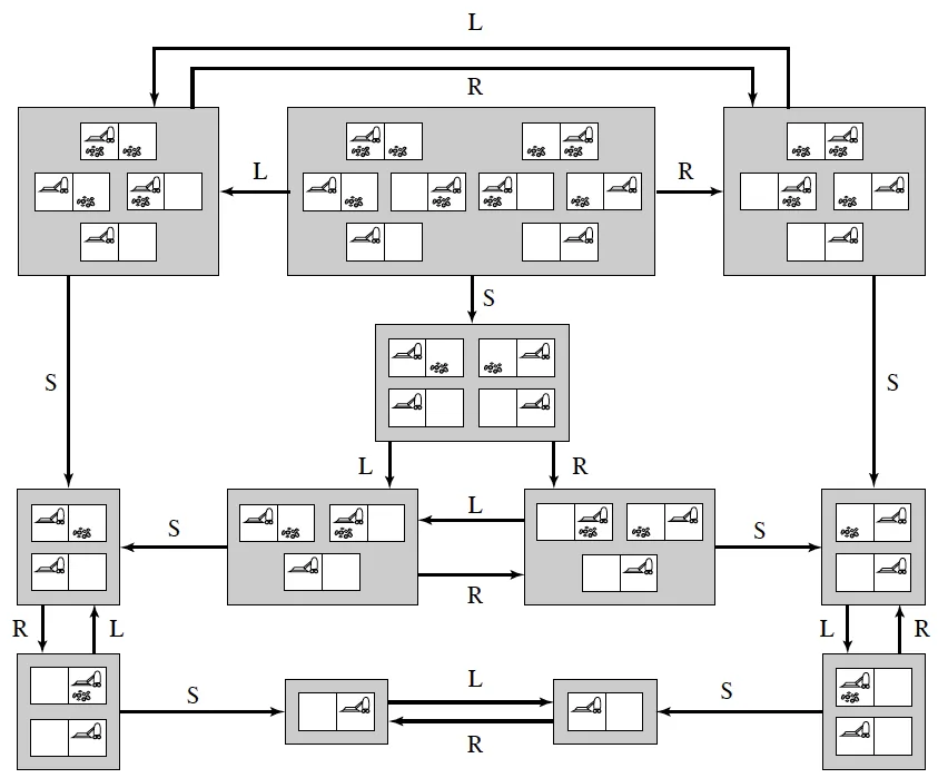
Searching with partial observations

Slippery Vacuum World without global sensor

don't know where it is
use Belief-State Space (possible physical states)
$O(N)$ → $O(2^N)$

Incremental Belief-State Search

find a solution that works for state 1
check if it works for another state
- If not, go back and find an alternative solution for state 1
similar to AND-OR search

Online Search

combine computation and action
Works good in
- Dynamic or semi-dynamic domains
- Stochastic domains
- Exploration problem in unknown environments
impossible to take into account all possible contingencies(可能性，意外)
The agent maintains a map of the environment
- Updated based on percept input
- use map to decide next action
- difference with e.g. A*
  - online search can only expand the node it is in local map

Example: Maze

reach a goal with minimal cost
Competitive ratio
- compare the cost of the solution path if search space is known
Can be infinite
- agent accidentally reaches dead ends
Assume Safely explorable
- some goal state is reachable from every reachable state
No algorithm can avoid dead ends in all state spaces

Online DFS

Untried: action not yet tried
Unbacktracked: state not yet backtracked(尚未走回去過的state)
Worst case each node is visited twice
- online iterative deepening approach solves this problem

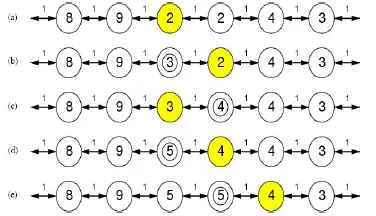
Online Local Search

Hill-climbing is already online
- only store one state
Bad performance due to local maxima
- can not random restart in online version
Solution
- Random walk introduces exploration
  - time complexity is exponential
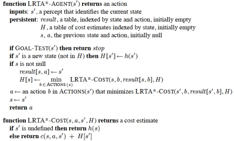
- Learning real-time A* (LRTA*)
  - Add memory to hill climbing
  - Store current best estimate H(s) of cost to reach goal
  - H(s) is initially = h(s), the least possible cost
    - updated with experience
  - O(n^2)

Chap05 Adversarial Search(game)

In 1948, Turing met Donald Michie and competed with him in writing a simple chess-playing algorithm
The Historical Match in 1997
- Kasparov vs. Deep Blue
Games are idealization of worlds
- the world state is fully accessible
- the (small number of) actions are well‐defined
- uncertainty exists due to moves of the opponent
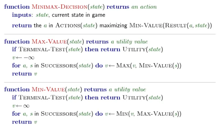
Minimax
MaxMax(negamax)
- Advantage of over MiniMax
  - Consistent view: maximize scores
  - Subroutine Min is not required

Implementation of Pruning

Pass the current best score to child nodes
Stop searching and return when a branch exceeds the score from the parent

Alpha-Beta search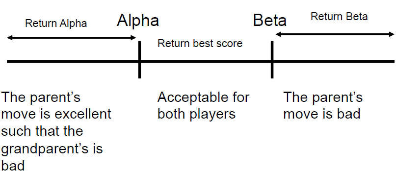

only use about $O(b^(d/2))$ time

Improvement of A-B search

Search good move first
- Heuristic move ordering
  - Checkmate
  - Killer
    - The move that results in beta pruning earlier
- Iterative deepening
  - good moves in the search depth = N are usually good in depth = N+1
- Principle variation search
  - NegaScout
- Zero‐window search
  - expect returned value = -3 with beta pruning
  - if return -4, real value is between [4, ∞], search again
Reuse scores for duplicate nodes
- Transposition table
  - save board layout and score in hash table
Risky estimation of best score
- Null-move search
  - give up a move once
  - returned score serves as an estimate value for pruning
Extend the depth for some leaf nodes
- Score may not be acccurate if the board situation is not quiescent(靜止，即交換棋子的過程告一段落)
  - A series of recapture moves
  - Checkmates
- Horizon Effect
  - threat will be happened in the deep depth
- Singular Extension
  - give more depth to some nodes
prune without further consideration
- Forward Pruning
- Probabilistic Cut
  - pruning nodes which are merely possible to be good move
End Game
- retrograde(倒推)
  - reverse the rules to chess to do unmoves

Stochastic game

Chance Layer added to search tree
- possible states after stochastic action
expect value
- sum all values in chance layer with probability
- $(4 \times 0.5 + 6 \times 0.5) \div 2 = 5$

Bridge

inperfect information
- belief state
GIB program
- monte-carlo(handle randomness well)
- explaination-based generalization
  - only consider high-card or low-card

evaluation function has error

error is not independent(probably all children)
consider mean and variance

Time-limited search

if utility of node expansion is not higher than their cost(time), do not expand

Chap06 Constraint Satisfaction Problems(CSP)

specialization of general search
state is defined by variables with values from domain
Example: Map-Coloring
- Variables = set of regions
- Domains = {red,green,blue}
- Constraints: adjacent regions must have different colors
Solutions are complete and consistent assignments
- consistent: assignment that does not violate any constraint
Binary CSP: each constraint relates only two variables
- Constraint graph: vertexs are variables, edges are constraints

CSP types

Discrete variables
- finite domains
  - n variables, domain size d → $O(d^n)$ complete assignments
  - Ex. Boolean CSPs(NP-complete)
- infinite domains(integers, strings, ...)
  - use constraint language, e.g., x1 + 5 ≤ x3
  - Ex. job scheduling, variables are start/end days for each job
Continuous variables
- linear constraints solvable in polynomial time by linear programming
  - Ex. quadratic programming
- Ex. start/end times for observations
No algorithm exist for solving general nonliear constraints

constraint types

Unary constraints involve a single variable
- SA ≠ red
Binary constraints involve pairs of variables,
- SA ≠ WA
3 or more variables
- cryptarithmetic(覆面算，用英文字母來取代0至9的數字) column constraints
Preferences (soft constraints)
- green is better than red

Real-World CSPs

Assignment problems
- who teaches what class
Timetabling problems
- which class is offered when and where
Transportation scheduling

Standard Search Formulation (Incrementally)

Every solution will be found in depth n → prefer to use depth-first search
Path is irrelevant, so can also use complete-state formulation of local search
b = (n-l)d at depth = l, hence $n! \times dn$ leaves

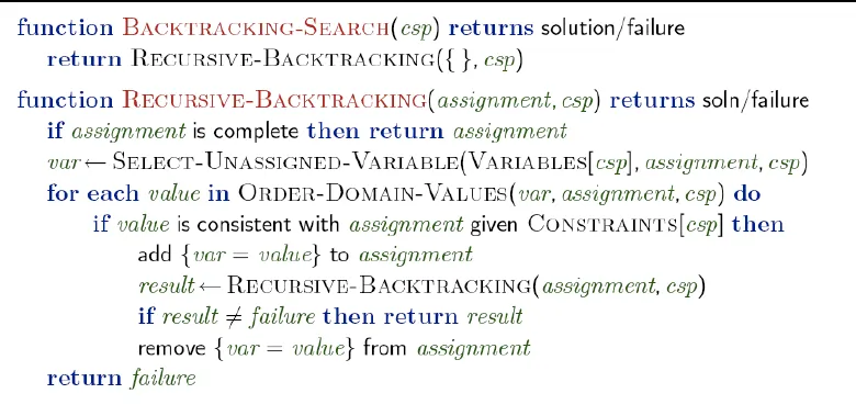
Backtracking Search

depth-first search for CSPs with assigning one variable per action
basic uninformed algorithm for CSP
by wiki: 回溯法採用試錯的思想，它嘗試分步的去解決一個問題。在分步解決問題的過程中，當它通過嘗試發現現有的分步答案不能得到有效的正確的解答的時候，它將取消上一步甚至是上幾步的計算，再通過其它的可能的分步解答再次嘗試尋找問題的答案
Can solve n-queens for n ≈ 25

Improve Backtracking

General-purpose methods can give huge gains in speed
- variable assignment order
  - Most constrained variable(minimum remaining values (MRV) heuristic)
    - choose the variable with the fewest legal values
  - Most constraining variable(degree heuristic)
    - choose the variable with the most constraints
- value assignment order
  - Least Constraining Value
    - choose the value that make the fewest values be deleted in the remaining variables
    - give the most flexibility
- detect inevitable failure early
  - Forward Checking
    - Keep track of legal values for unassigned variables
    - Terminate search when any variable has no legal value
    - Only consider arc-consistency
      - the graph already has arc-consistency need not do this
    - Maintain Arc consistency (MAC)
Combining these heuristics can solve n-queens for n ≈ 1000

Intelligent Backtracking

Chronological Backtracking
- when the search fails, back up to the preceding decision point(多選題)
  - the most recent decision point is revisited
- equals to DFS
Backjumping
- backtracks to the most recent variable in the conflict set(variables that caused the failure)

Constraint Propagation(傳播限制)

early detection for all failures
local consistency(graph)
- variable: node, binary constraint: arc
transform all n-ary constraints to binary one
Node consistency(1-consistency)
- all values in domain satisfy unary constraints
Arc consistency(2-consistency)
- all values in domain satisfy binary constraints
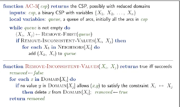
- Algorithm: AC3
Path consistency
- 若xi, xj的domain，可以使第三個variable xk的domain滿足{xi, xk}和{xj, xk}的consistency
If variable X loses a value, neighbors of X need to be rechecked (detect inconsistency)
- Ex. Arc Consistency
- REMOVE-INCONSISTENT-VALUE: 如果Xi的Domain中，有無法達成 Xi↔Xj 這個條件的值，則刪除

k-Consistency

for any set of k-1 variables and for any consistent assignment to those variables, a consistent value can always be assigned to the k-th variable
只要有任何k-1個確定值的變數，必有一確定值可以放在第k個變數
A graph is strongly k-consistent if it is k-consistent and is also (k-1)-consistent, (k-2)-consistent, … 1-consistent
- guarantee to find solution in O(n^2d)
- but establishing strongly k-consistent graph take exponential time
commonly use 2 or 3 consistency in pratice

Subproblem

suppose each subproblem has c variables, total n variables
worst-case cost: $\frac{n}{c}\times d^{c}$
cost is far better
- n = 80, d = 2, c =20 → $2^80$ → $4 \times 2^{20}$

Local Search for CSPs

allow unsatisfied states
value selection by min-conflicts heuristic
- h(n) = total number of violated constraints
Evaluation function of N-queen
- h = number of pairs of queens that are attacking each other
- can solve n-queens for n ≈ 10000000 (O(n) = constant) with high probability
variant
- allow variable move to the same score
- prevent to select recently choosed variables
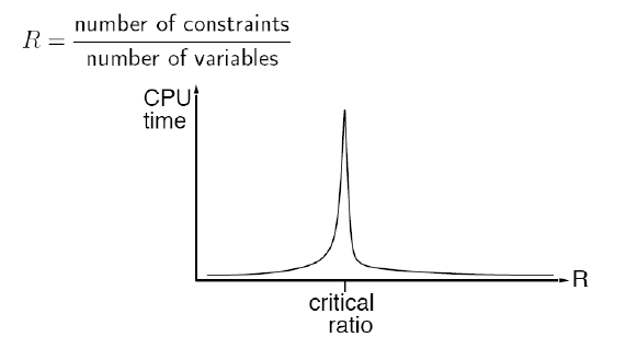
Critial Ratio of local search for CSP
- In certain ratio, it's hard to solve CSP by local search
- 剛剛好的限制條件(答案數過少)→數獨題目
Advantage
- can easily change into online setting

Theorem of Tree-Structed CSP

if the constraint graph has no loops, CSP can be solve in $O(nd^2)$ time, which is far better than general CSP($O(d^n)$)
1. make problem arc-consistent O(n)
2. assign value O(d^2)
Algorithm
1. transform problem to a tree
2. for i = n to 2, do REMOVE-INCONSISTENT-VALUE(Parent(Xi), Xi)
3. for i = 1 to n, assign Xi consistently

Graph reduced to tree

constraint graph
- given fixed value for some of the nodes to make remaining a tree
- if small cut is found, it is efficient
tree decomposition
- 把一部分的圖形變成一個大的node，把這些大的node合成一顆樹
- 規則
  3. 若兩個variables本來有相連，他們必須出現在同一個subgraph至少一次
  1. 若一個variable出現多次，則那些subgraph要彼此相連
  2. 每個variable至少要出現一次
- make subgraph as small as possible
  - tree width: size of the largest subproblem
- $O(nd^{w+1})$, w = tree width

Breaking symmetry

reduce search space by n! by breaking symmetry
- A: red, B: blue ↔ A:blue, B:red
- set A < B
  - only one solution A:blue, B:red \

Summary

CSPs are a special kind of problem
- states defined by values of a fixed set of variables
- goal test defined by constraints on variable values
Variable ordering and value selection heuristics help significantly
Iterative min-conflicts is usually effective in practice

Chap07 Logical Agents

Can agent prove theorems?

David Hilbert (1862-1943)

“Hilbert’s Program” [1920]
- mechanize mathematics
- The consistency of more complicated systems, such as real analysis, could be proven by simpler systems
- consistency of all of mathematics could be reduced to basic arithmetic
- 所有數學應用一種統一的嚴格形式化的語言，並且按照一套嚴格的規則來使用
Gödel showed that this is impossible
Automatic theorem proving simply tries to mechanize what can be mechanized

Gödel's Incompleteness Theorem (Kurt Gödel, 1931)

In any consistent formalization of mathematics that is sufficiently strong to define the concept of natural numbers, one can construct a statement that can be neither proved nor disproved within that system(任何相容的形式系統，只要蘊涵皮亞諾算術公理，就可以在其中構造在體系中不能被證明的真命題，因此通過推演不能得到所有真命題（即體系是不完備的）。)
No consistent system can be used to prove its own consistency (can not simultaneously be true and false) 任何相容的形式系統，只要蘊涵皮亞諾算術公理，它就不能用於證明它本身的相容性

《戈德爾不完備定理》，董世平
任一個證明，都必須從某一個公設系統出發。對於自然數我們最常用的公設系統就是皮亞諾公設 (Peano Axioms)，這些公設中最複雜而且困難的，（不僅對一般的高中，大學生如此，對邏輯學家亦如此），就是大名鼎鼎的「數學歸納法」。藉著數學歸納法及其他的公設，我們可證明「質數有無窮多個」，問題是「是否所有有關自然數的敘述，只要是對的，就可由皮亞諾公設出發，而得到證明呢？」也就是「皮亞諾公設是否完備?」若皮亞諾公設具有完備性，那麼所有有關自然數的敘述，若是對的，就可由皮亞諾公設證明。
由戈德爾不完備定理而得的一個結論，就是「皮亞諾公設是不完備的！」有些關於自然數的敘述是對的，但皮亞諾公設無法證明它，戈德爾的證明也的確告訴我們如何找到這個敘述。事實上，由戈德爾的證明，我們可得一個算則，給我們一個公設系統，我們就可按此算則，而得到一個算術句型，再經過適當的編譯 (compile)，即可成為此系統內的一個句型，而此句型在此系統內為真，卻無法在此系統內被證明，所以也許我們會覺得皮亞諾公設不具有完備性，這是它的缺點，我們應當找另一個具有完備性的公設系統來代替它，但不完備定理告訴我們，「任何一個具有一致性的公設化系統皆是不完備的！」這也就是為什麼雖然大家明知皮亞諾公設是不完備的，但這個公設系統仍是被普遍的使用，因為任何其他系統，也都是不完備的。也許我們再退一步，皮亞諾公設固然不具有完備性，我們至少可要求它具有一致性吧！也就是皮亞諾公設所證明的，一定是真的，可惜，這一點也做不到，由不完備定理可得另一個結論就是「在皮亞諾公設系統內將無法證明它的一致性！」從某一方面來說，你須要假設比「皮亞諾公設是一致的」更強或相等的假設，你才能證明皮亞諾公設的一致性，當然我們若須要更強的假設，也就須要更大的信心去相信它是對的。同樣的，皮亞諾公設也沒那麼特殊，就像不完備性的結果一樣，由戈德爾不完備定理，任一個足夠強的公設系統，皆無法證明它本身的一致性。

第一不完備定理
- 任何一個足夠強的一致公設系統，必定是不完備的
- 即除非這個系統很簡單，(所以能敘述的不多)，或是包含矛盾的，否則必有一真的敘述不能被證明
第二不完備定理
- 任何一個足夠強的一致公設系統，必無法證明本身的一致性
- 所以除非這個系統很簡單，否則你若在此系統性，證明了本身的一致性，反而已顯出它是不一致的

哥德爾證明：任何無矛盾的公理體系，只要包含初等算術的陳述，則必定存在一個不可判定命題，用這組公理不能判定其真假。也就是說，「無矛盾」和「完備」是不能同時滿足的！這便是聞名於世的哥德爾不完全性定理。

從程式人的角度證明「哥德爾不完備定理」

knowledge-based agents

use logical sentences(邏緝式) to infer conclusions about the world

KnowledgeBase Agent

processes of reasoning that operate on representation of knowledge
knowledge base
- set of sentences (axioms)
  - given without derived from other sentences
- tell agent how to operate in this environment
inference
- derive new sentences from old

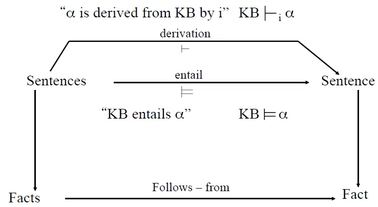
Terminology

α ╞ β: α entails β
- if there is a model that α is true, β is also true
- α is a stronger assertion than β
- x = 0 ╞ xy = 0
An interpretation is a model for a theory if it assigns true to each formula in the set
A formula is satisfiable if it is true in at least one model
- m satisfies α → m is a model of α
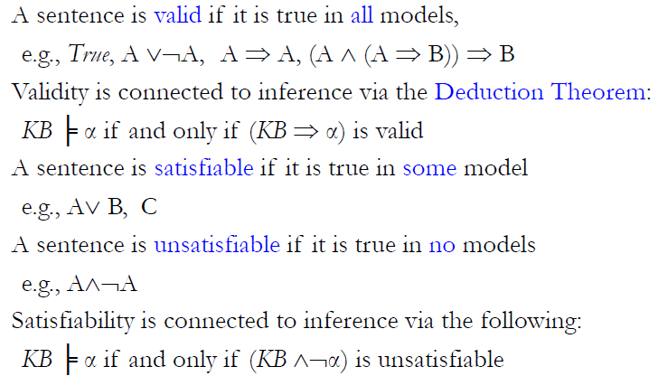
A formula is valid if
- it is true under all possible interpretations
- Its negation is not satisfiable

Validity and Satisfiability

演繹定理聲稱如果公式 F 演繹自 E，則蘊涵 E → F 是可證明的(就是或它可以自空集推導出來)。用符號表示，如果 $E \vdash F$ ，則 $\vdash E \rightarrow F $
- KB ╞ α if and only if (KB → α) is valid
Relation to Inference
- KB ╞ α if and only if (KB → ~α) is unsatisfiable

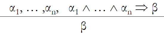
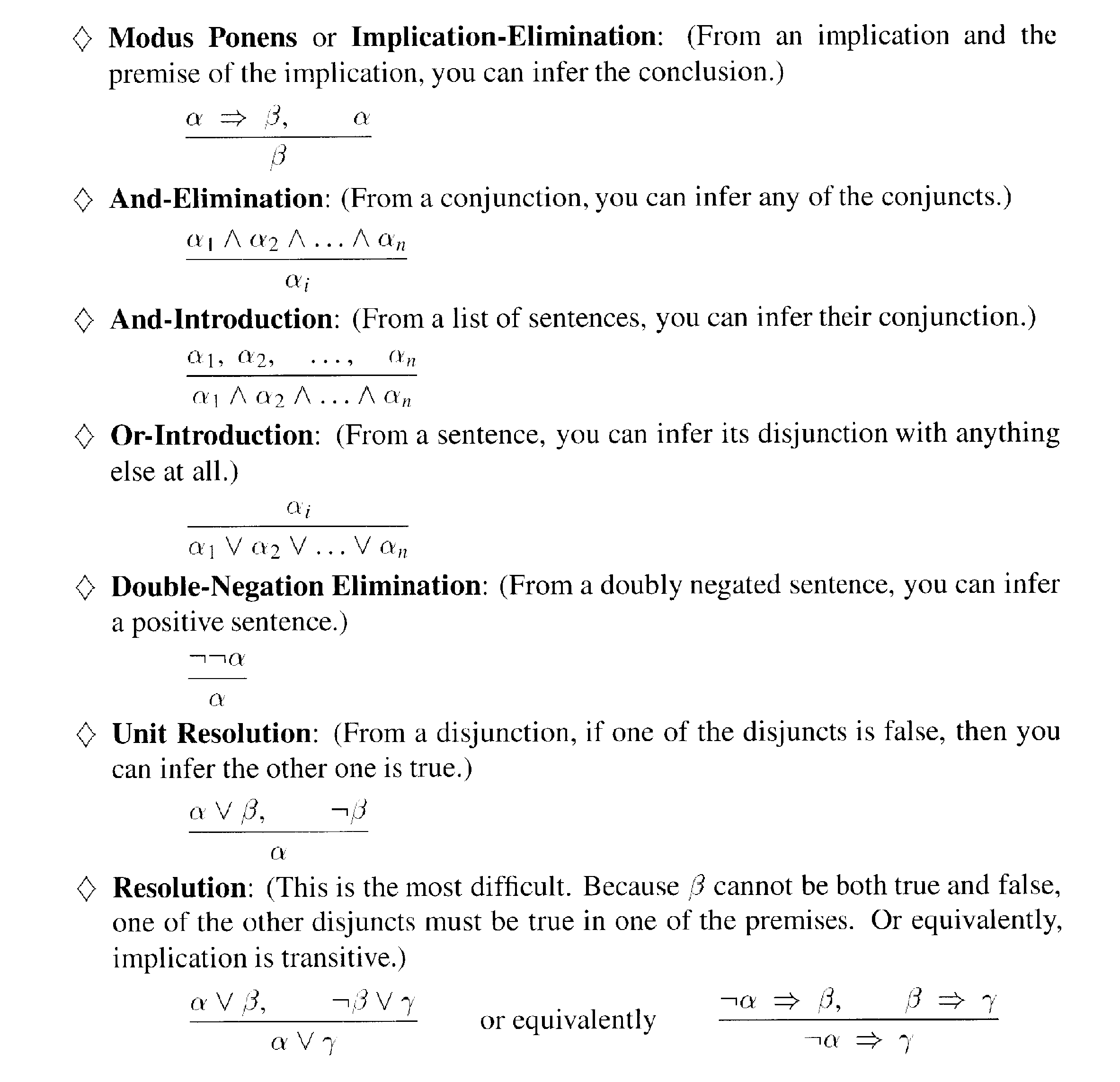
Inference Rules

modus ponenes(推論法則)
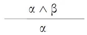
and-elimination
Propositional Rule of Inference

Propositional Logic

Syntax and Semantics

symbol
- assigned by true or false
- literal: symbol or ~symbol
- constants: True(always true), False(always false)
connectives
- or(disjunction), and(conjunction)

Proof Methods

Application of inference rules
- generation proof sentence by inference
- Proof = a sequence of inference rule applications
  - Can use inference rules as operators in a standard search algorithm
- Typically require transformation
Model checking
- truth table enumeration
  - exponential time
- improved backtracking
  - e.g., Davis-Putnam-Logemann-Loveland (DPLL)
- heuristic search in model space (sound but incomplete)
  - e.g., min-conflicts-like hill-climbing algorithms

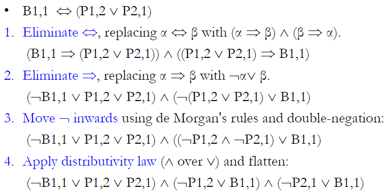
Conjunctive Normal Form

any propositional formula can be transform to conjunctive normal form
(or or ...) and (or or ...) and (or or ...) ...
each () is a clause
Convert normal formula to CNF

Example: Wumpus

Using Resolution(歸結) inference rule
- $\frac{\Gamma_1 \cup\left{ \ell\right} ,,,, \Gamma_2 \cup\left{ \overline{\ell}\right} }{\Gamma_1 \cup\Gamma_2}|\ell|$

Testing Validity

truth tables
- exponential time
Resolution
Forward & backward chaining
DPLL
Local Search Methods
- Complete backtracking search algorithms
  - DPLL algorithm (Davis, Putnam, Logemann, Loveland)
- Incomplete local search algorithms
  - WalkSAT algorithm

Resolution

Sound
- inference that derives only entailed sentences
- if KB is true, then any sentence α derived from KB by sound inference is also true
Completeness
- if it can derive any sentence that is entailed

Resolution refutation is sound(可靠) and refutation complete(完備) for propositional logic

If we derive a contradiction, then the conclusion follows from the axioms
If we can’t apply any more, then the conclusion cannot be proved from the axioms
A formal system S is refutation-complete if it is able to derive false from every unsatisfiable set of formulas
KB ╞ α if and only if (KB → ~α) is unsatisfiable
- proof KB ╞ α by showing (KB ^ ~α) is unsatisfiable

Binary Resolution Step
For any two clauses C1 and C2

Find a literal L1 in C1 that is complementary to a literal L2 in C2
Delete L1 and L2 from C1 and C2 respectively
Construct the disjunction of the remaining clauses
The constructed clause is a resolvent of C1 and C
Ex. $\frac{a \vee b, \quad \neg a \vee c}{b \vee c}$
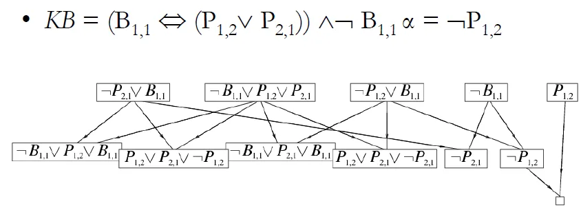
put P1,2 into clause set to check whether "~P1,2 is in KB"
- Proof by contradiction：The derivation of [] indicates that the database of clauses is inconsistent
  - P1,2 is in KB

Resolution algorithm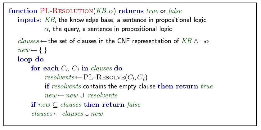

Propositional Horn Clauses

At most one positive literal
Satisfiability can be tested in linear time
Resolution is fast for Horn clauses, and very slow in non-Horn clauses
- resolve two horns → one horn
Basis of Prolog
- Head:-body
inference done by forward and backward chaining

Forward and Backward Chaining

Horn Form (restricted)
- KB = conjunction of Horn clauses
Horn clause =
- proposition symbol, or
- (conjunction of symbols) => symbol
Modus Ponens(肯定前件)(for Horn Form): complete for Horn KBs
- used with forward chaining or backward chaining
- run in linear time
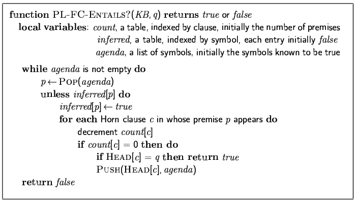
Forward Chaining
- fire any rule whose premises are satisfied in the KB, add its conclusion to the KB, until query is found
Backward chaining
- work backwards from the query q to prove q by BC, check if q is known already, or prove all premises of q
- Avoid loops
  - check if new subgoal is already on the goal stack
- Avoid repeated work
  - check new subgoal

Forward vs. backward chaining

both sound and complete for Horn KB
FC is data-driven, automatic, unconscious processing
- e.g., object recognition, routine decisions
- May do lots of work that is irrelevant to the goal
BC is goal-driven, appropriate for problem-solving,
- e.g., Where are my keys? How do I get into a PhD program?
- Complexity of BC can be much less than linear in size of KB

Davis-Putnam Procedure(DPLL)

Introduced by Davis & Putnam in 1960
Modified by Davis, Logemann & Loveland in 1962 [DPLL]
- Resolution rule replaced by splitting rule
- Trades space for time

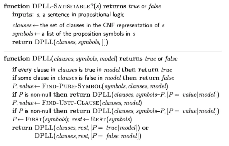
DPLL

recursive, depth-first enumeration of possible models
- determine if an input CNF is satisfiable with the following

Improvements

Early termination
- A clause is true if any literal is true(用or相連)
- A sentence is false if any clause is false(因為用and相連)
Unit clause heuristic
- only one non-false literal in the clause
  - The only literal in a unit clause must be true
- a clause with just one literal (i.e. all other literals are assigned false)
Pure symbol heuristic
- a symbol that always appears with the same sign in all clauses
- Ex. A and ~A would not both appear in a sentence if A is pure
- Make a pure symbol literal true
  - 在全設成true時, KB自然是true

DPLL(continue)

Unit propagation
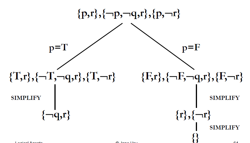
Example
backtracking search for a model of the formula
Interpretations are examined in a sequential manner
- DPLL(KB, p←TRUE) is testing interpretations if p is TRUE
- DPLL(KB, p←FALSE) is testing interpretations if p is FALSE
For each interpretation, a reason is found that the formula is false in it
•Such a sequential search of interpretations is very fast
–DPLL is much faster than propositional resolution for non-Horn clauses
•Very fast data structures developed
•Popular for hardware verification

Chap08 First-Order Logic

How Do Humans Process Knowledge?

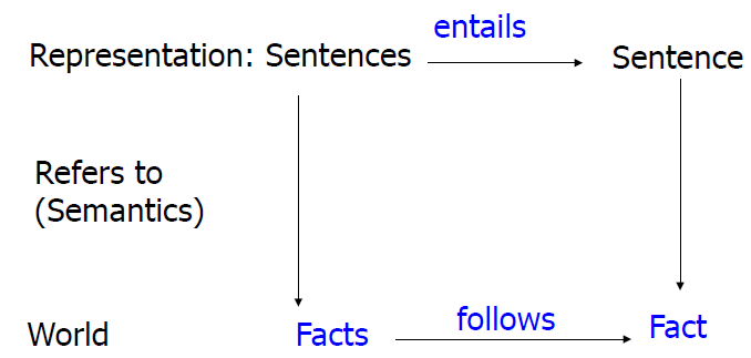
people process the words to form some kind of nonverbal representation, which we call memory
Logic as a representation of the World

Sapir-Whorf Hypothesis

The language we speak profoundly influences the way in which we think and make decisions
- setting up the category structure by which we divide up the world into different sorts of objects
  - Eskimos have many words for snow and thus experience snow in a different way
Two way to think(??)
- aware of the distinctions only by learning the words
- distinctions emerge from individual experience and become matched with the words

Logics

A logic consists of the following:
- A formal system describing states of affairs
  - Syntax
  - Semantics
- proof theory – a set of rules for deducing the entailments of a set of sentences
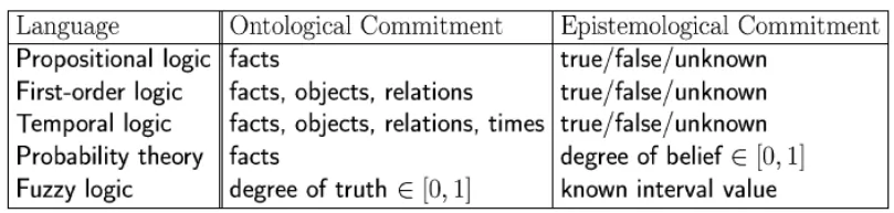
Ontological commitments
- FOL: facts, objects, relations
- Probability theory: facts
Epistemological commitments
- What an agent believes about facts, e.g. FOL: true/false/unknown probability theory: degree of belief [0..1]

Logical Truth and Belief

Ontological Commitment: What exists in the world — TRUTH
Epistemoligical Commitment: What an agent believes about facts — BELIEF

(重複？)
Terminology

Propositional constants: true, false
Interpretation
- Truth assignments to propositional symbols
- Truth-functional meaning of logical connectives
Theory: a set of formulas in logic
An interpretation is a model for a theory if it assigns true to each formula in the set.
- A formula is satisfiable if it has (at least) a model
- A formula is valid if
- It is true under all possible interpretations
  – Its negation is not satisfiable.

Propositional Logic

Propositional logic is declarative
Propositional logic allows partial/disjunctive/negated information
- (unlike most data structures and databases)
Propositional logic is compositional:
- meaning of B1,1 ∧ P1,2 is derived from meaning of B1,1 and of P1,2
Meaning in propositional logic is context-independent
- (unlike natural language, where meaning depends on context)
Propositional logic has very limited expressive power
- unlike natural language
- E.g., cannot say "pits cause breezes in adjacent squares“
  - except by writing one sentence for each square

wumpus-world agent using propositional logic
→ 64 distinct proposition symbols, 155 sentences
contains "physics" sentences for every single square
a lot of clauses

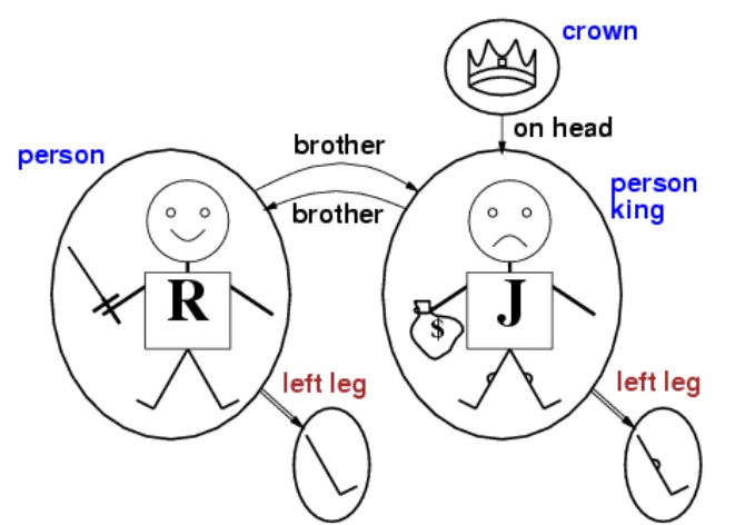
First-Order Logic

propositional logic assumes the world contains facts
first-order logic assumes the world contains
- Objects: people, houses, numbers, colors, baseball games, wars, …
- Relations: red, round, prime, brother of, bigger than, part of, comes between, …
- Functions: father of, best friend, one more than, plus, …

Syntax of FOL: Basic elements

Constants
- KingJohn, 2, NUS,...
Predicates
- Brother, >,...
Functions
- Sqrt, LeftLegOf,...
Variables
- x, y, a, b,...
Connectives
- ¬, ⇒, ∧, ∨, ⇔
Equality
- =
Quantifiers
- ∀, ∃

Atomic sentences

Atomic sentence = predicate (term1,...,termn) or term1 = term2
Term = function (term1,...,termn) or constant or variable
Examples
- King John is the brother of Richard the Lion Heart
  - Brother(KingJohn,RichardTheLionheart)
- Richard’s left leg is longer than King John’s
  - Greater-than(Length(LeftLegOf(Richard)),Length(LeftLegOf(KingJohn)))

Complex sentences

Complex sentences are made from atomic sentences using connectives
- ¬S,S1 ∧ S2,S1 ∨ S2,S1 ⇒ S2,S1 ⇔ S2
Examples
- Sibling(KingJohn,Richard) ⇒ Sibling(Richard,KingJohn)

Truth in First-Order Logic(??)

Sentences are true with respect to a model and an interpretation
Model
- objects (domain elements)
- relations among objects
Interpretation specifies referents for
- constant symbols → objects
- predicate symbols → relations
- function symbols → functional relations
An atomic sentence predicate(term1,...,termn) is true iff the objects referred to by term1,...,termn are in the relation referred to by predicate

Models for FOL

We can enumerate the models for a given KB vocabulary
- For each number of domain elements n from 1 to ∞
Computing entailment by enumerating the models is not easy

Knowledge Engineering in FOL

Identify the task
Assemble the relevant knowledge
Decide on a vocabulary of predicates, functions, and constants
Encode general knowledge about the domain
Encode a description of the specific problem instance
Pose queries to the inference procedure and get answers
Debug the knowledge base

Domain: Electronic Circuits(Adder)

Identify the task
- Does the circuit actually add properly?
Assemble the relevant knowledge
- Composed of wires and gates
- Types of gates (AND, OR, XOR, NOT)
- Connections between terminals
- Irrelevant: size, shape, color, cost of gates
Decide on a vocabulary
- Alternatives
  - Type(X1) = XOR
  - Type(X1, XOR)
  - XOR(X1)
General Domain Knowledge
- ∀t1,t2 Connected(t1, t2) ⇒ Signal(t1) = Signal(t2)
- ∀t Signal(t) = 1 ∨ Signal(t) = 0
- 1 ≠ 0
- ∀t1,t2 Connected(t1, t2) ⇒ Connected(t2, t1)
- ∀g Type(g) = OR ⇒ Signal(Out(1,g)) = 1 ⇔ ∃n Signal(In(n,g)) = 1
- ∀g Type(g) = AND ⇒ Signal(Out(1,g)) = 0 ⇔ ∃n Signal(In(n,g)) = 0
- g Type(g) = XOR ⇒ Signal(Out(1,g)) = 1 ⇔ Signal(In(1,g)) ≠ Signal(In2,g))
- ∀g Type(g) = NOT ⇒ Signal(Out(1,g)) ≠ Signal(In(1,g))
Specific Problem Instance
- Type(X1) = XOR Type(X2) = XOR
- Type(A1) = AND Type(A2) = AND
- Type(O1) = OR
- Connected(Out(1,X1),In(1,X2)) Connected(In(1,C1),In(1,X1))
- Connected(Out(1,X1),In(2,A2)) Connected(In(1,C1),In(1,A1))
- Connected(Out(1,A2),In(1,O1)) Connected(In(2,C1),In(2,X1))
- Connected(Out(1,A1),In(2,O1)) Connected(In(2,C1),In(2,A1))
- Connected(Out(1,X2),Out(1,C1)) Connected(In(3,C1),In(2,X2))
- Connected(Out(1,O1),Out(2,C1)) Connected(In(3,C1),In(1,A2))
Query
- What are the possible sets of values of all the terminals for the adder circuit?
- ∃i1,i2,i3,o1,o2 Signal(In(1,C_1)) = i1 ∧ Signal(In(2,C1)) = i2 ∧ Signal(In(3,C1)) = i3 ∧ Signal(Out(1,C1)) = o1 ∧ Signal(Out(2,C1)) = o2

Domain: Kinship(親屬關係)

Brothers are siblings
- ∀x,y Brother(x,y) ⇔ Sibling(x,y)
One's mother is one's female parent
- ∀m,c Mother(c) = m ⇔ (Female(m) ∧ Parent(m,c))
“Sibling” is symmetric
- ∀x,y Sibling(x,y) ⇔ Sibling(y,x)
A first cousin is a child of a parent’s sibling
- ∀x,y FirstCousin(x,y) ⇔ ∃p,ps Parent(p,x) ∧ Sibling(ps,p) ∧ Parent(ps,y)

Domain: Set

∀s Set(s) ⇔ (s = {} ) ∨ (∃x,s2 Set(s2) ∧ s = {x|s2})
¬∃x,s {x|s} = {}
∀x,s x ∈ s ⇔ s = {x|s}
∀x,s x ∈ s ⇔ [ ∃y,s2} (s = {y|s2} ∧ (x = y ∨ x ∈ s2))]
∀s1,s2 s1 ⊆ s2 ⇔ (∀x x ∈ s1 ⇒ x ∈ s2)
∀s1,s2 (s1 = s2) ⇔ (s1 ⊆ s2 ∧ s2 ⊆ s1)
∀x,s1,s2 x ∈ (s1 ∩ s2) ⇔ (x ∈ s1 ∧ x ∈ s2)
∀x,s1,s2 x ∈ (s1 ∪ s2) ⇔ (x ∈ s1 ∨ x ∈ s2)

Universal Qantification

∀
- Everyone at NTU is smart
  - ∀x At(x,NTU) ⇒ Smart(x)
equivalent to the conjunction of instantiations(例證來源) of P
- At(KingJohn,NTU) ⇒ Smart(KingJohn) ∧ At(Richard,NTU) ⇒ Smart(Richard) ∧ At(Mary,NTU) ⇒ Smart(Mary) ...
Common Mistake
- Typically, ⇒ is the main connective with ∀
- Wrong: using ∧ as the main connective with ∀
- ∀x At(x,NTU) ∧ Smart(x) means “Everyone is at NTU and everyone is smart”

Existential Quantification

∃
- Someone at NTU is smart
  - ∃x At(x,NTU) ∧ Smart(x)
equivalent to the disjunction of instantiations of P
- At(KingJohn,NTU) ∧ Smart(KingJohn) ∨ At(Richard,NTU) ∧ Smart(Richard) ∨ At(Mary,NTU) ∧ Smart(Mary) ∨ ...
Typically, ∧ is the main connective with ∃
- Common mistake: using ⇒ as the main connective with ∃
- ∃x At(x,NTU) ⇒ Smart(x) is true if there is anyone who is not at NTU!

Properties of Quantifiers

∀x ∀y = ∀y ∀x
∃x ∃y = ∃y ∃x
∃x ∀y ≠ ∀y ∃x
- ∃x ∀y Loves(x,y)
  - “There is a person who loves everyone in the world”
- ∀y ∃x Loves(x,y)
  - “Everyone in the world is loved by at least one person”
Quantifier duality
- each can be expressed using the other
- ∀x Likes(x,IceCream) ↔ ¬∃x ¬Likes(x,IceCream)
- ∃x Likes(x,Broccoli) ↔ ¬∀x ¬Likes(x,Broccoli)

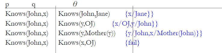
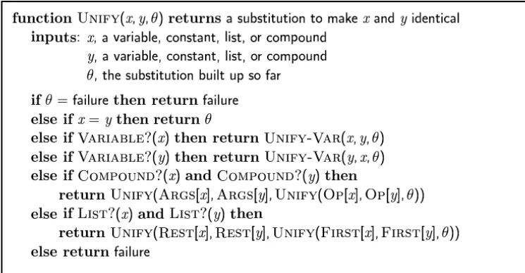
Unification

To unify Knows(John,x) and Knows(y,z)
- MGU = { y/John, x/z }
There is a single most general unifier (MGU) that is unique up to renaming of variables
We can get the inference immediately if we can find a substitution θ such that King(x) and Greedy(x) match King(John) and Greedy(y)
Unify(α,β) = θ if αθ = βθ
Standardizing apart eliminates overlap of variables
- Knows(z17,OJ)

Conversion to CNF

Everyone who loves all animals is loved by someone
∀x [∀y Animal(y) ⇒ Loves(x,y)] ⇒ [∃y Loves(y,x)]

Eliminate biconditionals and implications
∀x [¬∀y ¬Animal(y) ∨ Loves(x,y)] ∨ [∃y Loves(y,x)]
Move ¬ inwards: ¬∀x p ≡ ∃x ¬p, ¬ ∃x p ≡ ∀x ¬p
∀x [∃y ¬(¬Animal(y) ∨ Loves(x,y))] ∨ [∃y Loves(y,x)]
∀x [∃y ¬¬Animal(y) ∧ ¬Loves(x,y)] ∨ [∃y Loves(y,x)]
∀x [∃y Animal(y) ∧ ¬Loves(x,y)] ∨ [∃y Loves(y,x)]
Standardize variables: each quantifier should use a different one
∀x [∃y Animal(y) ∧ ¬Loves(x,y)] ∨ [∃z Loves(z,x)]
Skolemize: a more general form of existential instantiation
Each existential variable is replaced by a Skolem function of the enclosing universally quantified variables
∀x [Animal(F(x)) ∧ ¬Loves(x,F(x))] ∨ Loves(G(x),x)
Drop universal quantifiers
[Animal(F(x)) ∧ ¬Loves(x,F(x))] ∨ Loves(G(x),x)
Distribute ∨ over ∧
[Animal(F(x)) ∨ Loves(G(x),x)] ∧ [¬Loves(x,F(x)) ∨ Loves(G(x),x)]

First-order logic

objects and relations are semantic
syntax: constants, functions, predicates, equality, quantifiers
Increased expressive power: sufficient to define wumpus world

Reference

Jane Hsu 上課講義
Artificial Intelligence: A Modern Approach
http://aima.cs.berkeley.edu/instructors.html
http://www.cs.ubc.ca/~hkhosrav/ai/310-2011.html
https://en.wikibooks.org/wiki/Artificial_Intelligence

Introduction

Turing Test

Taxonomy of AI

The History of AI

Historical Achievements

Other Usage of AI

Chap02 Agents

Agents and environments

Rationality

Task Environment: PEAS

Environment types

Agent types

Chap03 Search

Problem-solving agents

Problem types

Problem formulation

Problem Domains

Implementation: States vs. Nodes

Search Property

Type of Search

Uninformed search (blind search)

Graph Search

Chap03b Informed Search

Inventing Better Heuristic Functions

Summary: all informed algorithms

Chap04 Beyond Classical Search

Local Search Algorithms

Hill climbing(爬山)

Simulated annealing

Local Beam Search

Genetic algorithms

Local search in continuous spaces

Searching with nondeterministic actions

Searching with partial observations

Online Search

Chap05 Adversarial Search(game)

Chap06 Constraint Satisfaction Problems(CSP)

Backtracking Search

Chap07 Logical Agents

Gödel's Incompleteness Theorem (Kurt Gödel, 1931)

knowledge-based agents

Terminology

Propositional Logic

Proof Methods

Testing Validity

Resolution

Propositional Horn Clauses

Forward and Backward Chaining

Davis-Putnam Procedure(DPLL)

Chap08 First-Order Logic

Reference