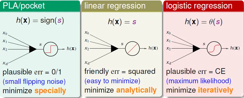
機器學習基石(下)
Chap09 Linear Regression
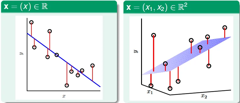
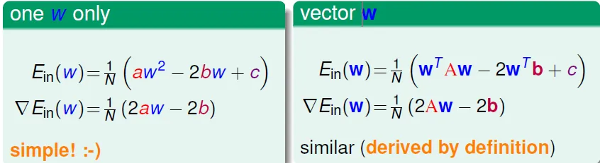
- 將w向量(參數)最佳化
- 直接用計算出的 Wx
- perceptron → output 只有 +1/-1
- regression → output 為數字
- 找最少誤差
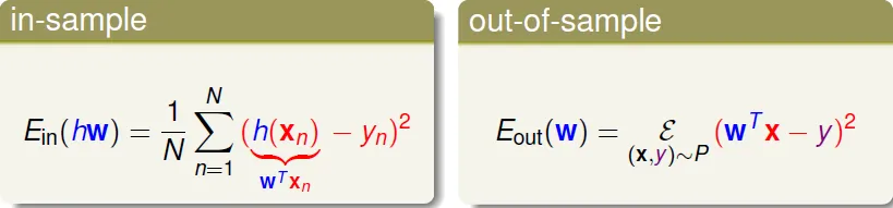
![]()
- wx 和 y 的誤差平方
- Ein: 取平均, Eout: 取期望值
![]()
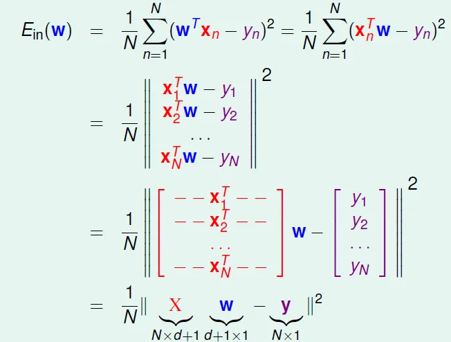
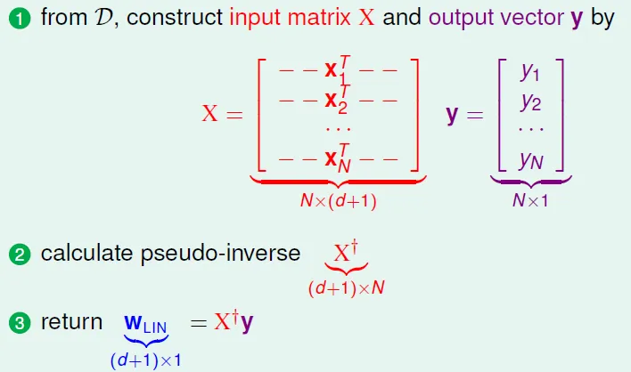
轉換成矩陣形式(最後一行的X, y, w都是矩陣)
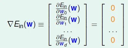
Ein(w)函數性質
- continuous
- differeniable
- convex(凸)
- 可以找到最低點(使Ein微分 = 0的w)
![]()
- 因為 A 為 $X^tX$ 的形式,必為symmetric matrix,可直接做微分
![]()
- 因為 A 為 $X^tX$ 的形式,必為symmetric matrix,可直接做微分
計算W 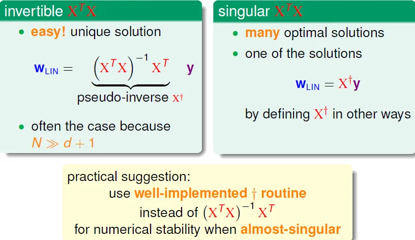
- 若A invertible,可直接求inverse
- 若非,則用X十字架(pseudo inverse)
linear regression algorithm(easy)
Is it "learning algorithm"?
- No → 直接計算所得的解
- Yes → good Ein and Eout(finite $d_vc$), pseudo-inverse
- 可視為迭代進行(用矩陣一次算出)
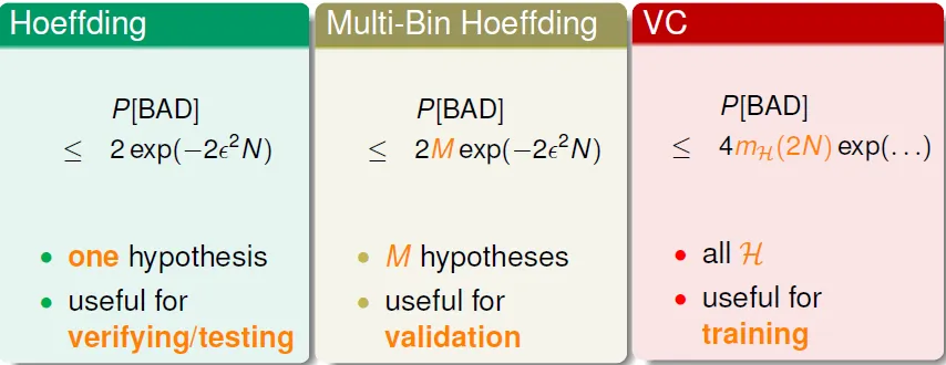
"Simpler-than-VC" Guarantee
可證Ein會小於????
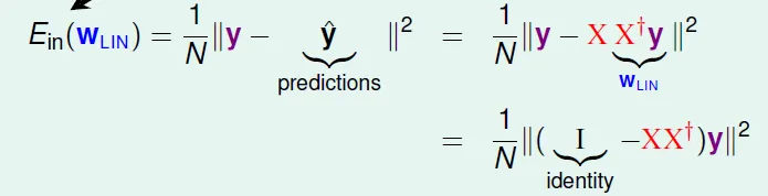
預測值 $\hat{y} = Xw = XX^{-1}y = Hy$
定義 hat matrix $H = XX^{-1}$
Hat Matrix in Geometry
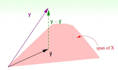
- 預測值 $\hat{y}$ 被限制在X的span上 ($\hat{y} = WX$)
- 最小誤差會出現在y - $\hat{y}$ 與 span of X 垂直時
- H 將向量投影至span of X上
- I-H : 投影至與 span of X 垂直的向量 (即為誤差: y - $\hat{y}$)
- 可以發現 I-H 對角線上的值之和 trace(I - H) = N - (d + 1)
- 其物理意義為在N維空間投影至d+1維空間
- 可以發現 I-H 對角線上的值之和 trace(I - H) = N - (d + 1)
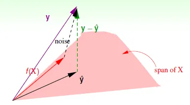
- with noise
![]()
- f(x) + noise → y
- f(x) 為正確的 y
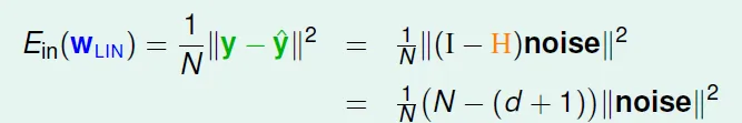
- noise * (I-H) = y - $\hat{y}$
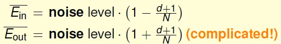
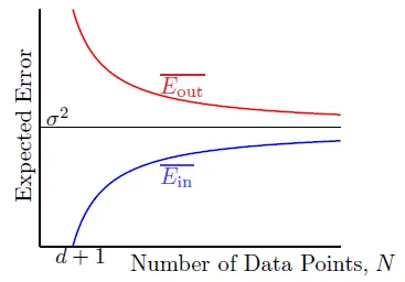
- 可算出Ein和noise的關係: N變大時, Eout↓, Ein↑, noise level收斂在σ^2
![]()
![]()
![]()
- Eout可用類似方法證明
- expected generalization error(= Eout - Ein): 2(d+1)/N
- f(x) + noise → y
Usage
Run Linear Regression Algo(efficient) and set initial w = $w^T_{lin}$ to speed up the perceptron learning
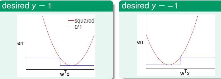
- 誤差大小(看面積): Square Error > 0/1 Error
![]()
- regression產生的 W 比 classification 的誤差更大,但計算時間較短
![]()
- regression產生的 W 比 classification 的誤差更大,但計算時間較短
Chap 10 Logistic Regression
Heart attack prediction
Not every people with bad condition will have heart attack
→ only P(Heart attack | x) probability
→ look it as noise
若機率 P(+1|X) > 1/2,則當成 +1,其他output當作noise 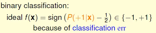
‘soft’ binary classification: f(x) = P(+1|x)
- ideal data: probabilty ↔ we have only noisy data(+1 or -1)
- the same data as perceptron, but different target function
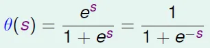
Logistic Hypothesis
- smooth, monotonic, sigmoid(S形) function
![]()
![]()
- 0 <= θ(x) <= 1
- θ(x) + θ(-x) = 1
- θ(-∞) = 0, θ(0) = 0.5, θ(∞) = 1
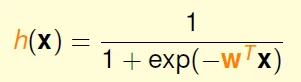
- 令 $h(x) = θ(w^Tx)$
![]()
Likelihood
if h ~= f, [h 產生 y 的機率] 接近 [f 產生 y 的機率(其值通常大於產生其他output的機率)]
猜測:若能找到h, 其產生的output和f很像的話(也就是和data的output很像), 那h也會和f很像 → 成功學習
g = argmax_h likelihood(h) 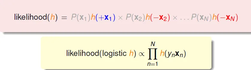
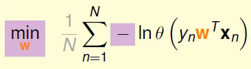
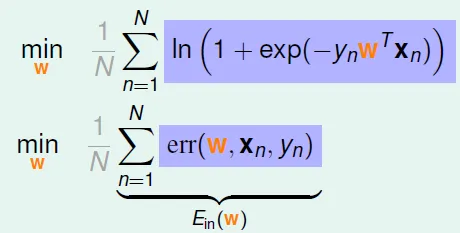
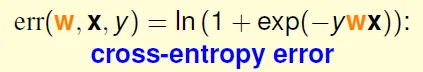
Cross-Entropy Error
- 因為 h(x) = θ(wTx)
- h(x) = h(-x)
- 最高可能性 = max Π h(ynxn)
- Π = 連乘
- = max ln Π θ(ynwxn)
- 轉換成θ,取ln
- = max Σ ln θ(ynwxn)
- ln Π = Σ ln
- = min 1/N x Σ -lnθ(ynwxn)
![]()
- 乘1/N, 加上min和負號
- 代入θ公式, Ein =
![]()
- 此函式即為 Cross-Entropy Error
![]()
- 此函式即為 Cross-Entropy Error
Minimize Cross-Entropy Error
find ∇Ein(w) = 0 to find min(Ein) 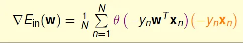
- 使所有θ項都為0
- only if all ynwxn >> 0
- 需要linear-seqerable data
- Σ(-ynxn) = 0
- non-linear equation of w
→ 都不好算
solve it by PLA
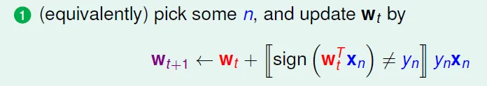
- 若有錯則更新,正確則不變($w^t = w^{t+1}$)
![]()
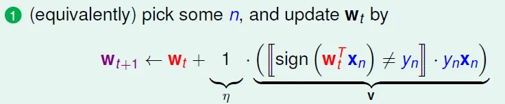
- 加入參數η,為更新的幅度倍率(本來為1)
![]()
- v 代表原本的式子
- 用 (xn, yn) 更新的大小: $θ(-y_nw^Tx_n)$
PLA smoothing
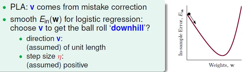
- 更新時就是在往Ein較低的方向走
- v為方向, η為幅度
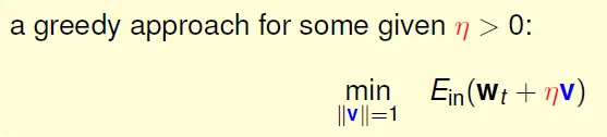
- Greedy
- 每次更新時調整η, 使Ein最小
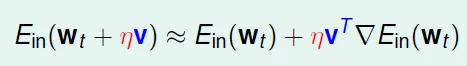
![]()
- η夠小的時候,可用泰勒展開式
![]()
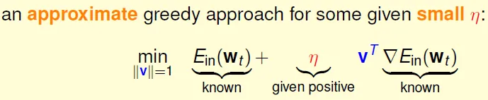
- 估算出的greedy更新公式
![]()
- η夠小的時候,可用泰勒展開式
- 每次更新時調整η, 使Ein最小
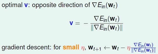
- Gradient Descent
![]()
- 最優的v是與梯度相反的方向,如果一條直線的斜率k>0,說明向右是上升的方向,應該向左走
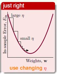
- 距離谷底較遠(位置較高)時,步幅(η)大些比較好;接近谷底時,步幅小些比較好
- 梯度的數值大小間接反映距離谷底的遠近
![]()
- 希望步幅與梯度大小成正比
- wt+1 ← wt - η∇Ein(wt)
- 梯度的數值大小間接反映距離谷底的遠近
Update Time
- decide wt+1 by all data → O(N) time
- Can logistic regression with O(1) time per iteration(like PLA)?
→ use one of data instead of all data
→ Stochastic Gradient Descent
Stochastic Gradient Descent (SGD)
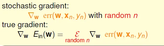
- 隨機選其中一筆資料來對 w 進行更新
- 進行足夠多的更新後,平均的隨機梯度與平均的真實梯度近似相等
- η often use 0.1
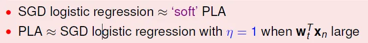
- compare PLA and SGD
![]()
- SGD is more flexible than PLA
Chap 11 Linear Models
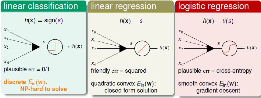
can linear regression or logistic regression help linear classification?
 ys: classification correctness score
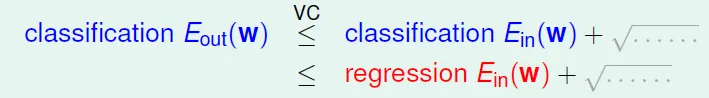
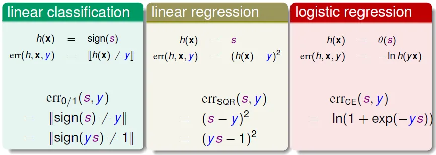
Error functions 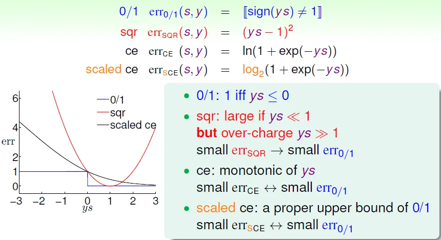
- small 0/1 error $\nRightarrow$ small square error
- small err SQR → small err 0/1
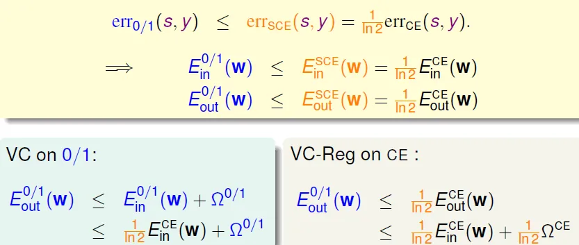
- small Err CE → small Err 0/1
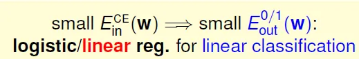
- ** small cross entropy error implies small classification error **
![]()
![]()
- small err SCE(scaled cross entropy) ↔ small err 0/1
- ** small cross entropy error implies small classification error **
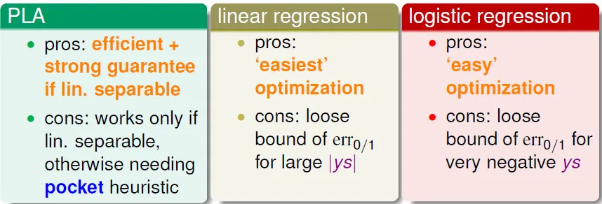
- PLA
- 優點:在數據線性可分時高效且準確
- 缺點:只有在數據線性可分時才可行,否則需要借助POCKET算法(沒有理論保證)
- linear regression
- 優點:最簡單的優化(直接利用矩陣運算工具)
- 缺點:ys 的值較大時,與 0/1 error 相差較大
- 線性回歸得到的結果w可作為其他算法的初始值
- logistic regression
- 優點:比較容易優化(梯度下降)
- 缺點:ys 是非常小的負數時,與 0/1 error 相差較大
- 實際中,logistic回歸用於分類的效果優於線性回歸的方法和POCKET算法
Multiclass Classification - meta algorithms
- One-Versus-All (OVA) Decomposition
- 對每個分類做logistic regression(共N個),選分數y最高的
- 優點:prediction有效率,學習時可平行處理
- 缺點:output種類很多時,數據往往非常不平衡(x 遠大於 o),會嚴重影響訓練準確性
- multinomial logistic regression 考慮了這個問題
- One versus One (OVO)
![]()
- 共有 N(N-1)/2 個 perceptron,投票決定
- 優點: training有效率(每個perceptron較小), 可以使用 binary classification 的方法
- 缺點: O(K^2) space
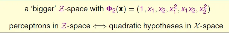
Chap 12 Nonlinear Transformation
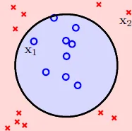
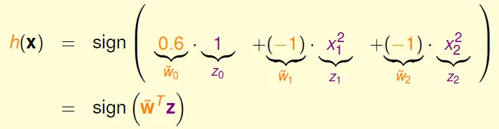
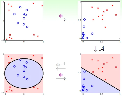
座標系轉換
- 將非線性的h(x)轉成線性
- circular separable in X → linear separable in Z
![]()
![]()
- 可在X做出任何二次曲線的Z
![]()
- circular separable in X → linear separable in Z
- transform data X to Z to train easily
![]()
- (xn, yn) → (zn = ϕ(xn), yn)
- train w by (z, y)
- g(x) = sign(ϕ(x)w) (= sign(wz))
- 代價
- O(Q^d)
- Q次方座標系, d個參數(x, y)
- $d_{vc}$ 隨 Q 成長
- O(Q^d)
力量愈強,代價愈大(可能會overfit)(見Chap13)
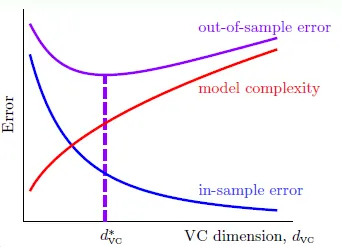
有效學習的條件
- Ein(g) 約等於 Eout(g)
- Ein(g)足夠小
當模型很簡單時(dvc 很小),我們更容易滿足1. 而不容易滿足2. ;反之,模型很複雜時(dvc很大),更容易滿足2. 而不容易滿足1.
→ 次方愈高,hypothesis set 包含愈多、愈複雜,Eout更偏離,也對數據擬合得更充分,Ein 更小 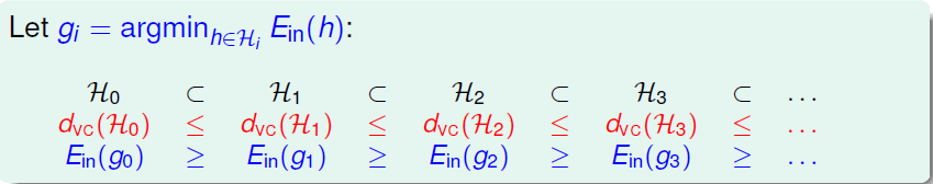
安全的方法: 先算低次方, 若結果已足夠好就不用繼續尋找
實務上的機器學習,通常都不會使用太高維度的learning
linear model first: simple, efficient, safe, and workable!
Legendre Polynomials Transform: 互為正交的函式(?),用來做transform效果較好
Chap 13 Overfitting
overfitting: **lower Ein, higher Eout **
右側為overfitting, 左側為underfitting
Case Study
target function 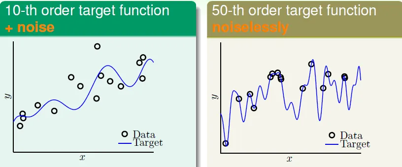
try 2nd order and 10th order function 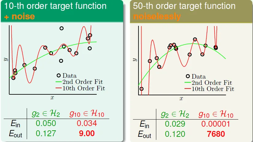
- 左側: H10 performance is not good even if original function is 10th-order
- 右側: even if no noise, there are still overfitting in H10
- hypothesis complexity acts like noise
- philosophy: 以退為進
- 絕聖棄智,其效百倍,絕巧棄利,error無有
雖然H10在N大的時候Eout較低,但在N小的時候Eout非常大 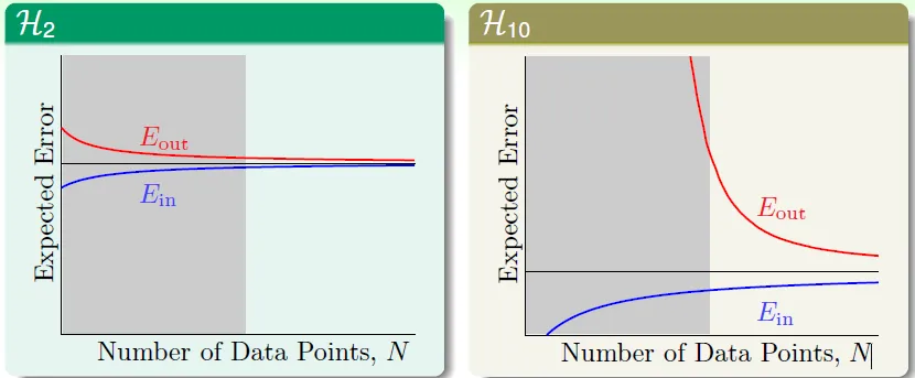
→ 資料不夠多(N小)的時候,不能用太複雜的hypothesis
實驗 noise 對 overfit 的影響
- noise ε with variance σ^2
- normal distributed iid
- red area has more overfit
![]()
- 造成overfit的原因

- deterministic noise
- 最好的hypothesis和target function的差異(depends on H)
- hypothesis complexity愈大,deterministic noise愈小
- stochastic noise
- N改變時,noise level對noise的影響
- 不是固定值、不能改善
- example: sample error
overfit的四個原因
- data size ↓
- stochastic noise ↑
- deterministic noise ↑
- hypothesis set的power ↑
類比成開車 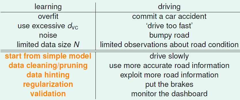
Overfit是很常發生的!
Data Cleaning/Pruning:
對於有些"奇怪"的data
- 改成自己認為是對的output (data cleaning)
- 移除資料 (data pruning)
Data Hinting:
用已有的知識處理原有的data,產生新的data(不是偷看!),適合於資料量不足時(Ex. 手寫辨識,可稍微旋轉、平移),要注意新data的比例是否符合現實情況
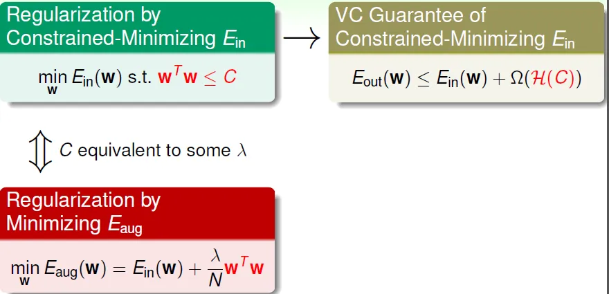
Chap14 Regularization
Regularization: 設條件(constraint) 降低 hypothesis set 的 complexity
| 對H10改動(= H2') | complexity |
|---|---|
| w3~w10為0 | H2' == H2 |
| w0~w10其中3個不為0 | H2 < H2' < H10 |
| wi的和小於一固定值 H(C)=sum(w^2)<=C | soft and smooth structure, e.g. H(0) < H(11.26) < H(∞) = H10 |
限制參數大小: NP-hard to solve 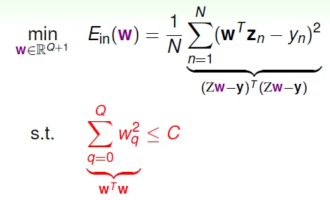
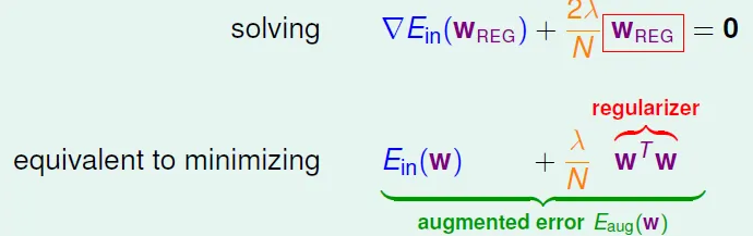
Lagrange Multiplier 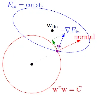
- min(Ein):朝梯度的反方向
- -▽Ein(W)為更新的向量
- W為原點到指定點的向量
- 只找出在紅色圓(限制)內的最佳解,即紅色圓上與$W_{lin}$最近的點
- $W_{lin}$為linear regression的解
- W與-▽Ein(W)平行的時候
![]()
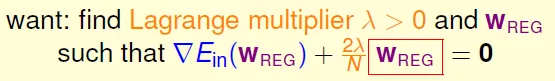
可以藉由設不同的 λ 來產生 W,此時 λ 和 H(C) 的 C 相似,用來限制參數
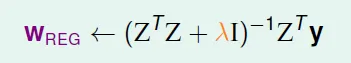
- Ridge Regression (similar to linear regression)
![]()
- Augmented Error
- solve min(Eaug) (unconstrained) is easier than solve min(Ein)(constrained)
- 積分後得到regularizer$w^Tw$
![]()
- wREG = argmin(w) Eaug(w)
- weight-decay
- Penalize large weights using penalties
- λ↑ → perfer shorter w → effective C↓
- λ 對應到 C
![]()
只需一點regularization就有效 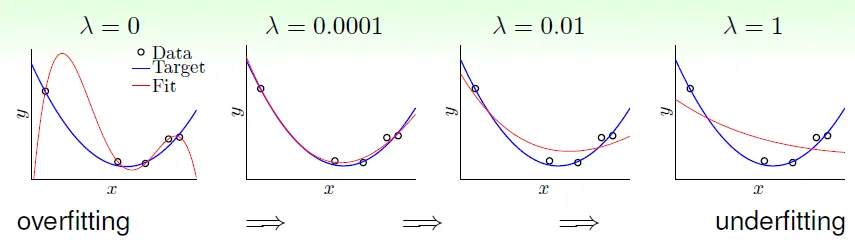
regularizer只限制單一hypothesis的complexity,不像VC bound整個hypothesis set都限制,所以Eaug比Ein更接近Eout 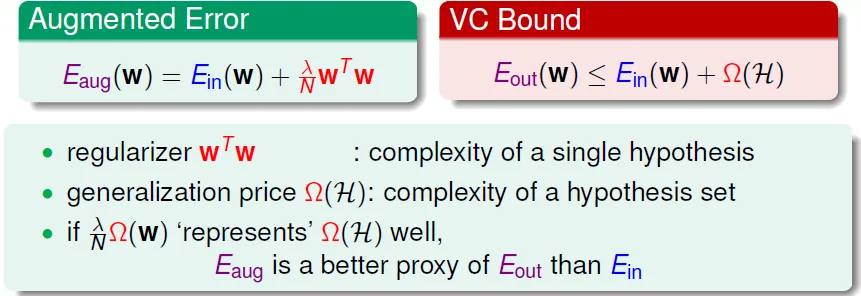
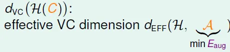
Effective VC Dimension of Eaug
- dVC(H) = d + 1
- 實際的 dvc 更小(被λ限制),但不好證明
![]()
General Regularizers 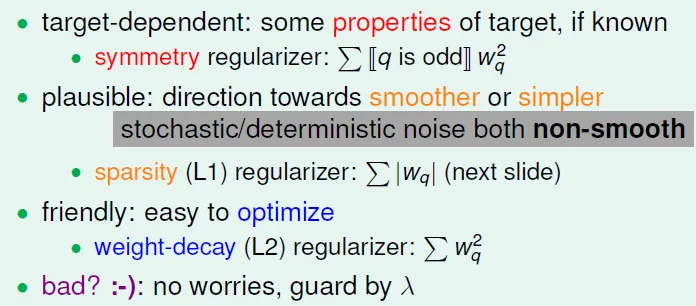
- target-dependent
- 用target function的性質來限制
- plausible(合理的)
- 預期比較平滑、簡單的hypothesis,因為noise是較不平滑的
- L1(sparsity regularizer): regularizer = Σ|wq|
- friendly(easy to use)
- L2(weight-decay regularizer): regularizer = Σ$w_q^2$
- comparison: error → user-dependent, plausible, friendly
- augmented error = error + regulizer
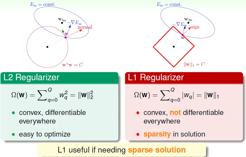 L1 useful when need sparse solution(有許多零的w, 因w最終會落到正方形的頂點),L1即表示限制函數為一次方
noise愈多,需要的regularization愈多 ↔ more bumpy road, putting brakes more 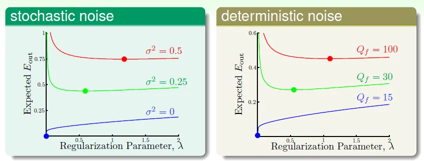
Conclusion:
正規化用來減少hypothesis的complexity,避免overfit,用wTw作regulizer(L2),以λ為參數調整正規化的程度(即L2圓的大小,L1正方形的大小),通常λ不會太大
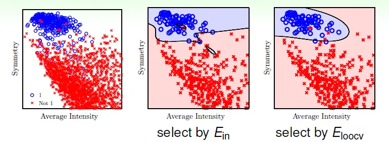
Chap15 Validation
So Many Models can choose, so use validation to check which is good choice
selecting by E_in is dangerous(can't reflect Eout)
selecting by E_test is infeasible and cheating(not easy to get test data)
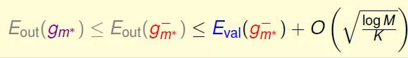
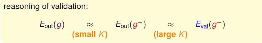
$E_{val}$: legal cheating
- 將data分成train和validation二部分
- 用train學習,用valid測試
在許多切割(fold)之中,找$E_{val}$最小的hypothesis,並用這個hypothesis和全部的data算出g 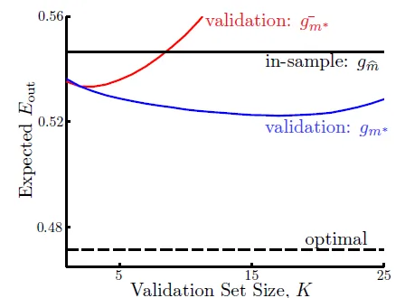
- $g_m^{-}$ 為 validation data 算出的g
![]()
- find balance of validation data size
![]()
- leave-one-out cross validation ($E_{loocv}$)
- 每次只用一個資料作validation(K = 1)
- often called ‘almost unbiased estimate of Eout’
![]()
- 缺點:計算太多(一個model要train N次, N為資料個數)
- 改善:切成n塊(通常5fold, 10fold)
- leave-one-out cross validation ($E_{loocv}$)
選擇 - 先選要測試的models,再用validation選出最好的
- all training models: select among hypotheses(初賽)
- all validation schemes: select among finalists(複賽)
- all testing methods: just evaluate
- Still use test result(之前沒用過的data) for final benchmark, not best validation result
Chap16 Three Learning Principles
Occam's Razor
An explanation of the data should be made as simple as possible, but no simpler
用最簡單且有效的方法解釋資料
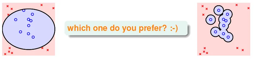
因為愈簡單的H 愈難分資料 → 可以分開資料時,有顯著性(若是用複雜模型,分開是很容易的)
→ linear first, always ask whether overfitting
Sampling Bias
抽樣誤差:抽樣非真正隨機
Ex. 1948電話民調,但電話當時昂貴
movie recommend system: When data have time sequential, should emphasize later data, do not use random data
Data Snooping
偷看資料(機器學習 → 人腦學習),會包含大腦所花的complexity 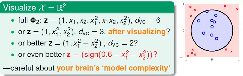
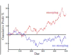
paper1: H1 works well on data D
paper2: find H2 and publish if better than H1 on D
....
→ bad generalization, cause overfit (if you torture the data long enough, it will confess)
→ 解決方法:不要先看paper,先提出自己的方法,再和已發表的方法比較
Conclusion
Three Related Fields
Three Theoretical Bounds
Three Linear Models
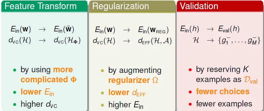
Three Key Tools: Feature Transform, Regularization, Validation
Three Future Directions(in ML techniques)

End~~
Reference
http://www.douban.com/doulist/3381853/
HTLin講義
Coursera